|
[With examples using SAGE Due to problems with java, sections that included dynamic figures are in revision. 3-22-2017 ] © 2002, revised 2014 M. Flashman
Introduction to the Sensible Calculus Program (SCP): The Sensible Calculus Program reflects work of over thirty years by Professor Martin Flashman that started in developing a thematic approach to the first year of calculus. (See [MAA,4].) Recognizing that a reform of the college precalculus function/algebra course would yield extra benefits in the success of calculus students, in about 1990 Professor Flashman expanded the vision of the program to include calculus preparation. The goal of the current project is the creation of a precalculus and a calculus textbook and a full calculus program with a consistent thematic and conceptual approach. The program will prepare students in the precalculus component for learning calculus by providing motivation, background, concept development, and opportunities for real learning. The calculus component will build on these foundations with an approach that extends precalculus maturation into calculus. Two (among several) distinctive features of the SCP approach will apply to both the precalculus and calculus components:
The
Agenda and Vision. Calculus projects over the
passed twenty five years have tried to improve the quality
of calculus instruction with approaches mixing
technology, pedagogical tactics, and curriculum
revisions. As a result there has been much progress in
rethinking the essential elements for a successful
calculus program, leading to a general acceptance of
many features of the reformed calculus agenda. Here is
a brief statement of the current agenda and vision
that the SCP addresses and which provide the
fundamental direction for The Sensible Calculus
Book.
The Sensible Calculus Program Approach: The SCP focuses on the themes of
differential equations [FL]
and estimation throughout the first year of calculus,
using modelling as a central motivation for
applications of the calculus [FL2].
In
the subsequent third semester or fourth quarter study
of the calculus of several variables and the vector
calculus these themes continue making an altogether
unified and coherent approach to calculus. These
themes and motivation have gained general approval
from many of today's best selling textbooks.
Unfortunately, there is no book today that succeeds in
presenting the calculus consistently with these
underlying principles. Along with thematic
consistency, an important and unique pedagogical
feature of the SCP text is the consistent use of
interpretations to provide meaning for calculus
concepts. Frequently examples of models or arguments
will be presented before more general applications and
proofs. This organization is based on the pedagogical
principle that students can understand the specific
and particular in experience and then generalize more
easily then they can understand a general proposition
or proof and the apply it to the particular.
Visualizations and Mapping Diagrams: Practically all major calculus concepts and techniques are interpreted with at least two views:
Many students in their first calculus course are still developing their basis for understanding the function concept. The combination of mapping diagrams with Cartesian graphs gives a dual approach to interpreting and visualizing functions that has been particularly helpful for these students. It also is a great aid in making sense of many calculus concepts and results, such as the chain rule and the differential. To make effective use of these visual tools the SCP employs them not merely in one or two instances as some current texts, but regularly invokes them in a variety of contexts [FL1]. This is central to the visually and conceptually balanced approach of the SCP. [See also [FL5], [S&J], and [G] for more on mapping diagrams.]
Using GeoGebra to do this:
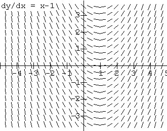
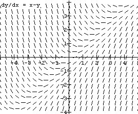
Differential Equations, Tangent
Fields, and Euler's Method. The use of tangent
(slope or direction) fields (see Figure
2 ) to visualize differential equations
and Euler's method for estimating solutions to initial
value problems (see Figure
3 ) are elements of the calculus curriculum that
have won general acceptance in that past ten years as
evidenced by their inclusion the current Advanced
Placement syllabus and the best selling texts.
Professor Flashman recognized the importance of these
tools for understanding the calculus early in his
development of The Sensible Calculus Program and has
worked over twenty years with students to find
presentations for these tools that are direct and easy
to follow. As a result of all this experience, The
Sensible Calculus Book combines an early
and extensive discussion of differential equations
with a visual approach through tangent fields [FL2]
and a numerical approach using Euler's method [FL1].
Throughout
the text the combined numeric and visual approaches
complement conventional symbolic discussions in
topics such as solving indefinite integrals,
motivating the definite integral and the Fundamental
Theorem of Calculus, finding precise function
solutions to initial value problems, and even more
advanced symbolic techniques such as the separating
variables. The dynamic features of SAGE
Using GeoGebra to do this: Estimating $f (1)$ from $y' = P( x,y ) = 2x -y $ with $f (0) = 2, N =4, x_N=1, dx = h = \frac 14$. You can change the values of the end points on the axis using the sliders or enter them in the boxes in the mapping diagram. Use the slider to change the value of $N$ up to $100$. You can change the function definition for the graph and the mapping diagram by entering a new function in the box. You can change the value of $f(a)$ directly in the spreadsheet cell. Click on the checkbox to show a slopefield with resolution also controlled by $N$
Another example using GeoGebra with $y'=P(x)$ as a function of $x$ alone: Estimating $f (2)$ from $y' = P( x ) = 2x + 1$ with $f (0) = 0, N = 10 , x_N=2, dx = h = \frac 15 =0.2$. You can change the values of the end points on the axis using the sliders or enter them in the boxes in the mapping diagram. Use the slider to change the value of $N$ up to $100$. You can change the function definition for the graph and the mapping diagram by entering a new function in the box. You can change the value of $f(a)$ directly in the spreadsheet cell.
Models: Connecting applications of the calculus to the real world is not new. For centuries the calculus has been used to understand and plan in science and engineering. In traditional calculus texts, geometric and physical applications appear as motivation primarily for the calculus concept of the derivative. Otherwise applications usually appear only after a technique or concept has been presented. The Sensible Calculus Book presents applications as a part of the modeling process in many contexts, both traditional and more contemporary, especially in economics and continuous probability. These contexts a threaded throughout the text, from the initial chapters on functions and the motivation of the derivative, to the first sections on differential equations and the introduction of both the indefinite and definite integrals, to the understanding of applications of the definite integral and the use of Taylor theory and concepts of infinite series. Frequently a model is presented for motivation and exploration before the calculus concept or technique as in the treatment of transcendental functions with differential equations. For example, a heuristic model for learning introduces a differential equation context. The basic premise is that the rate of learning is often a positive yet decreasing function of time, for instance i) $ L'(t) = \frac 1 t $ with $t \gt 0$ or ii) $L'(t) = \frac 1{t^2 + 1}$ . For the first equation, after a consideration of units and time scales, the boundary condition $L(1) = 0$ is established. Questions such as what will be the short and long run behavior of the learning function are investigated using tangent fields and Euler's method, as well as the derivative form of the Fundamental Theorem of Calculus. All this leads to a treatment of the natural logarithm function in the context of a differential equations model for learning. Likewise population (exponential growth and predator-prey) models motivate the exponential and trigonometric functions. All of these functions are treated with their traditional definitions as well. The object of the modeling approach is not to give formal rigorous treatments of these functions, but to show how the common functions arise and/or remain significant because they solve modelling problems expressed with differential equations. Second order differential equations and population models motivate the hyperbolic functions as student investigations. Taylor
Theory: Polynomial
functions and geometric series have been a part of the
calculus since the earliest work of Newon and Leibniz
that has developed into what is now described as
"Taylor theory." The Sensible Calculus
Book approaches Taylor theory as a
distinct and important part of calculus, not a mere
appendage at the end of a year's course treatment of
infinite series. The text's development is based on
the unifying themes of differential equations and
estimation. The calculus of Taylor polynomials (not
series) appears as a tool for approximating difficult
definite integrals such as $\int_0^1
e^{-x^2} dx$ with a sensible
control on the error. Estimating the solution to
differential equations such as $y'' = -y$ or $y''= y$ with
$y(0) = 1$ and $y'(0) = 0$ [ which characterize the cosine
and the hyperbolic cosine functions] provides
additional motivation for the convergence questions of
infinite series. Here again the problems we want to
solve are placed in the text before the
techniques or theory. Infinite sequences and series analysis discuss Taylor theory examples from the beginning along with the traditional examples of geometric and harmonic series. Historical connections to Newton's work in estimating the values of the natural logarithm illustrate how geometric series played a significant role in the showing the power of the early calculus for computation and estimation. Probability: One of the most important applications of the calculus in current science and engineering is its use as a foundation for understanding probability and statistics. The inclusion of a section or two on this application in the best selling texts demonstrates the increased awareness by authors and teachers of the importance of this application. The Sensible Calculus Book does more then include a token section on probability and calculus. It includes continuous probability in the development of concepts of both differential and integral calculus. Starting with a simple experiment of throwing a dart at a unit circle in the background pre-calculus sections, the text develops the distance from where the dart lands to the center of the circle as a random variable for further investigation. Trying to understand the distribution function for this random variable eventually leads to its density function, i.e., its derivative. The text treats probability concepts frequently as interpretations of the calculus. The evaluation form of the Fundamental Theorem of Calculus shows the integral relation of the distribution function to the density function. Other probability concepts, such as the median, mode, and mean are introduced with an appropriate calculus concept. The Sensible Calculus' unique approach to probability follows the philosophies of both the NCTM Standards and the California Framework that call for the exploration of probability concepts as a regularly encountered strand in the fabric of mathematics. Whether a student is planning to be an engineer, a physician, or some kind of scientist, one of the most useful parts of their mathematics training will be probability and statistics. Making probability more relevant throughout the course allows students to see the interaction of calculus with this universal application. It enriches their understanding of both subjects as well as showing the application of continuous mathematics to nondeterministic situations. Technology:
Though the SCP is not committed to any specific
technology, it presumes access to technology capable
of graphing and computation as well as some
programming features in the event that computation or
visual features are not predesigned in the
technology.The text is not driven by technology, but
it does presume (through its problem sets) that
students and teachers will use technology to explore
and enhance concepts as well as to solve
problems.
Example: Draft of Section on Tangent Fields. Example: Draft of Section on Euler's method . Examples: Draft of Section VI.A connecting differential equations to the exponential function and Section VI.B connecting differential equations to the natural logarithm function. Draft of VI.C connecting the natural logarithm and exponential functions.
Example: Draft of Section IX.A introducing Taylor Theory for $e^x$ with applications. Example: Draft of part of Section X.B Series: Some Key Examples.
[FL1] Flashman, Martin. "Computer Assisted Calculus And Themes for A Sensible Calculus," in Calculus and Computers: Toward a Curriculum for the 1990's, The Report of A Conference on Calculus and Computers Held at the University of California at Berkeley, August 24-27, 1989. [UMAP] Flashman, Martin. "A Sensible Calculus.," The UMAP Journal, Vol. 11, No. 2, Summer, 1990, pp. 93-96. [FL2] Flashman, Martin. "Using Computers to Make Integration More Visual with Tangent Fields," appearing in Proceedings of the Second Annual Conference on Technology in Collegiate Mathematics, Teaching and Learning with Technology of November 2-4, 1989, edited by Demana, Waits, and Harvey, Addison-Wesley, 1991. [FL3] Flashman, Martin. "Concepts to Drive Technology," in Proceedings of the Fifth Annual Conference on Technology in Collegiate Mathematics, November 12-15, 1992, edited by Lewis Lum, Addison-Wesley, 1994. [FL4] Flashman,
Martin. "Historical Motivation for a Calculus Course:
Barrow's Theorem," in Vita Mathematica: Historical
Research and Integration with Teaching, edited by
Ronald Calinger, MAA Notes, No. 40, 1996. [FL5] Flashman, Martin. Mapping Diagrams from A(lgebra) B(asics) to C(alculus) and D(ifferential) E(quation)s: [G] Gonick. Larry. The Cartoon Guide to Calculus, HarperCollins, 2012. [Excerpts from publisher.] [MAA,1] Committee on the Undergraduate Program in Mathematics, "Recommendations for a general Mathematical sciences program," Mathematical Association of America, Washington,1981. [MAA,2] Douglas, Ron, editor. Toward A Lean And Lively Calculus. MAA Notes, No. 6, 1986. [MAA,3] Steen, Lynn, editor. Calculus for a New Century: A Pump, Not A Filter. MAA Notes, No. 8, 1988. [MAA,4] Tucker, Thomas W., editor. Priming the Calculus Pump: Innovations and Resources. MAA Notes, No. 17, 1990. [MAA,5] Solow, Anita E., editor. Preparing for a New Calculus: Conference Proceedings. MAA Notes, No. 36, 1995. [MAA,6] Tucker, Alan C. and Leitzel, James R.C., editors. Assessing Calculus Reform Efforts: A Report to The Community. MAA Reports, No. 6, 1995. [MAA,7] Roberts, A. Wayne, editor. Calculus: The Dynamics of Change. MAA Notes, No. 36, 1996. [S&J]
Swann, Howard and Johnson, John. Prof. E. McSquared's
Calculus Primer, Janson Publications Inc., 1989.
|