 magnet.
See Figure ***. This magnet is very strong so that when I turn my back
to it and release a magnetic dart, the dart will be drawn to the board
and will land at random somewhere on the board.
 Example 0.C.1. Parked Cars. The mathematics in a model doesn't need to be very sophisticated. It can be as simple as a model for keeping track of how many cars are parked in a parking lot. Certainly what we need to do is count the cars that are there when we start out records and then keep a tally of the cars that enter and leave the lot.The simple statement that describes the relation for this model is that the number of cars in the parking lot at time t+k is the number of cars there at time t plus the number of cars that have parked between time t and time t+k less the number of cars that have left the lot during that same time period.
We can introduce some algebraic notation here. Let P(t) be the number of cars parked in the lot at time t, N(t,k) be the number of newly arrived cars that have parked between time t and time t+k, and L(t,k) be the number of cars that have left the parking lot between time t and time t+k. The rather simple abstraction relating these numbers would use the mathematical operations and structure of the number system. The model is then represented in the simple equation: P(t+k)=P(t) + N(t,k) - L(t,k). If we let the net change in the number of parked cars by DP = P(t+k) - P(t), the previous equation become DP=N(t,k) - L(t,k).
This simple (difference) equation model could be used just as easily to keep track of a population of birds in a forest, the amount of a water in a resevoir, or the amount of money in a checking account.
The fact that addition and subtraction in the number system works so easily and sensibly in representing the parked cars in the previous example may seem obvious. This next example demonstrates the choices made to process information in a model with mathematical structure.
Example 0.C.2. Batting Average. Suppose we are keeping track of a softball player's
batting average during a ten-game season. In the first seven games the
player was at bat 25 times and hit successfully 10 times for an average
of 10/25= .400 (= 2/5). The batter had a small hitting streak during the
last three games of the season with 6 hits for 10 times at bat, giving
an average for those three games of 6/10=.600 (= 3/5).
How do we determine
the player's batting average for the entire 10 game season? If the only
thing we consider is that the information needs to be combined in some
way, we have some choices to make.
We could add the two averages giving
an average of .400 + .600 = 2/5 + 3/5=1.000. Of course that doesn't make
sense, but how many times have you seen people just assume that the way
to combine numbers is to add them?
Maybe we should average the two averages. If we follow this suggestion, we add the two averages and then divide the sum by 2, giving an average of .500=1/2. At least this sounds more reasonable as the kind of number that we would recognize as describing the batter's success rate. But this method also has problems. Haven't we given too much credit in the overall average to the last 10 at bats?
What makes more sense in finding the player's overall batting average
is to determine the total number of the batter's hits and divide by the
total number of times at bat. Following this procedure we find the batter
had a total of 16 hits for 36 times at bat, or a batting average of .444
= 4/9. This is, in fact, the number that would be used to describe the
player's batting average for the season.
What does this example show us about modelling with numbers? You need to look at the numerical information's meaning in the model to determine what arithmetic procedure will fit the desired operation. In the example, to add the batting information for a batting average we did not add the batting averages, but added separately the number of hits and at-bats to find the final batting average.
N.B. As simple as it may be, it is important enough to note again that the use of mathematical operations in a model needs some careful thought to see that it is appropriate for the context. These choices may require some subtle analysis of the object or context and the mathematics to have the model be accurate and consistent.
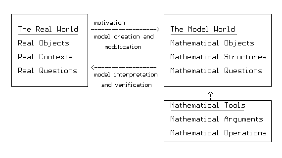
So here's one way to think about mathematical models. In the real world we have objects, contexts, and questions. Motivated by the real world, we create a model world with mathematics in which many aspects of the real world are true. We examine the world of the mathematical model with the special tools of mathematics to answer the mathematical model questions that correspond to the real world questions. If we can answer these mathematical questions, we take those answers and interpret them as being sensible in the real world. (This is possible because of the correspondence we establish through language between the real world and the mathematical model.)
We use the model answers, translated into the real world, to understand the real world, make real decisions, and plan real projects. We also can revise our model to accommodate changes in the real world and inconsistencies between our initial model results and what we find upon further investigations in the real world.
More Models, Contexts, Settings and Functions.
Besides the trip context discussed in our discussion of functions in
Chapter 0.B.2, there are many other common settings in which the function
concept can be used to understand the relation between variable quantities
in a mathematical model. Here are a few familiar and not so familiar situations
that will appear throughout our discussions in this book.
Experiments, Randomness and Probability (darts). In an overwhelming number of sciences the most common context involves the repetition of an experiment. During the experiment observations are made to find relations between variables that are controlled and measured during the experiment. The relation between the variables may be considered deterministic, controlled almost completely by the interrelations of the variables, or probabilistic [sometimes called stochastic], seemingly unpredictable and occurring randomly based on the information known prior to the experiment.
You may or may not have had previous experience with the concepts of probability, so for the time being let's assume you have only an informal and somewhat naive view. In particular when we say that an event E has a probability of p (say, for example, p = 1/4) of happening, where p is some real number between 0 and 1 you may interpret this as meaning roughly that if an experiment is repeated a large number of times, say N times (for example, N=1000 times), then you might expect the event E will occur approximately pN times ( for the example, 1/4 1000 = 250 times). It is convenient to write the probability of event E is p with Pr(E)=p.
The nature of a random (stochastic) variable may be a little abstract, so let's use a simple model to illustrate some probability concepts we'll use later in the course.
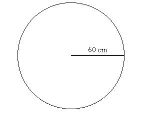
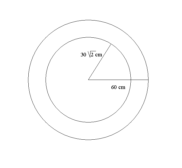
Example 0.C.3: Darts. Imagine a circular board of radius 60 centimeters
which is a powerful  magnet.
See Figure ***. This magnet is very strong so that when I turn my back
to it and release a magnetic dart, the dart will be drawn to the board
and will land at random somewhere on the board.
Let's assume the following
uniformity condition for simplicity: If we have any two regions on the
board of equal area then the dart would land in those regions about the
same number of times with a large number of throws. In other words,
the event of the dart falling in regions of equal area is equally probable
or equi-likely.
I'll throw a magnetic dart and mark where it lands
on the board. This is our basic experiment. Here are some typical questions
for this dart experiment:
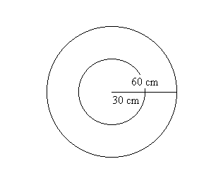
(i) If the board is divided into two regions by a concentric circle
of radius 30 and I repeat the experiment a large number of times, what
proportion of the markings is likely to fall in the inner region? See Figure
***.
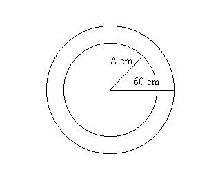
(ii) After repeating the experiment a large number of times, what proportion
of the markings is likely to fall within A cms of the center
where 0<A<60? See Figure ***.
 (iii) If the board is divided into four regions by concentric circles
of radius 15, 30, and 45 cm and I repeat the experiment a large number
of times, what proportion of the markings from the experiments is likely
to fall in
each of the regions?
(iv) If the board is divided into n regions by concentric circles of
radius (k/n) 60 cms with k = 1,2 ... n-1, and I repeat the experiment a
large number of times, what proportion of the markings from the experiments
is likely to fall in each of the regions?
There are many observations that might be recorded after a throw. As in any experiment, we will measure something that helps us answer a question. For each of the questions we posed one important piece of information we can observe is the dart's distance from the center of the circle. This measurement varies unpredictably with each throw, so it is called a random variable of the experiment. We'll use the letter R to denote the value of this random variable measuring the distance of the dart from the center of the circle. Each of the questions translates into a corresponding question about the random variable R. After throwing the dart, the random variable is measured and we can answer any of questions of where the dart landed by examining the value of R.
For example, from question (i) we would like to know: what proportion of the experiments is likely to give a value of R less than 30, i.e., R<30. The general question for (ii) would ask: what proportion of the experiments is likely where the value of R is less than A, i.e. R<A.
The probability that the dart would fall within the circle of radius
30 is determined by finding the probability that R<30. After looking
at Figure *** and some thought you should believe that this probability
can be measured by finding the ratio of the area inside the circle of radius
30 to the area of the circle of radius 60. Thus the probability that R
< 30 is ![]() .
.
Looking at the related question of the likelihood of the dart landing in the outer ring, we can analyze the areas of the regions in question to see the probability that 30<R is 3/4 .
Following the same type of reasoning, you should try to explain why
the probability that R<A for any A between 0 and 60 will be ![]() while the probability that A < R for R between 0 and 60 will be
while the probability that A < R for R between 0 and 60 will be ![]() .
These results allow us to answer the next
.
These results allow us to answer the next 
Question: For what choice of A will the probability of the dart following inside the circle of radius A be the same as the probability that dart will land outside the circle? [The answer to this question can be described as the median value of R.]
Answer: Let's assume we have found such a value for A. Then our
analysis shows that ![]() ,
... so after solving the algebra in this equation we can see that A must be
,
... so after solving the algebra in this equation we can see that A must be ![]() .
You can check that this value for A does answer the question correctly.
See Figure ***.
.
You can check that this value for A does answer the question correctly.
See Figure ***.
Extension: A slightly more interesting question is where to place
two concentric circles so that the probabilities of the dart landing in
either the inner circle, the outer ring, or the central ring are all equal
(namely 1/3). See Figure ***. From the previous discussion on the probability
of the dart falling inside a circle of radius A we have ![]() and likewise from the probability of the dart falling outside the circle
of radius B we have
and likewise from the probability of the dart falling outside the circle
of radius B we have ![]() .
With these equations we can conclude that A = 20sqrt(3) and B = 20sqrt(6).
.
With these equations we can conclude that A = 20sqrt(3) and B = 20sqrt(6).
The only additional general analysis we need to settle the third part of this question
is the probability of the dart landing inside the ring bounded by concentric
circles of radius B and A (assuming that B> A). As before we can use the
ratio of areas to measure the probability and you can check that this quantity
is precisely ![]() . This formula works out to be 1/3 with the previously found values for A and
B, so those values do make all three regions have equal area.
. This formula works out to be 1/3 with the previously found values for A and
B, so those values do make all three regions have equal area.
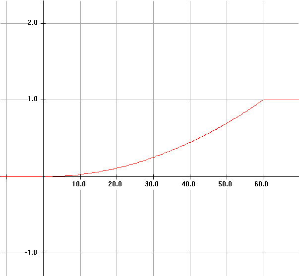
Notation: It is helpful and traditional to denote the probability
that a random variable R has a value <= A by F(A) where A in this
case is in the closed interval [0,60].
F is a function of A defined
on the interval [0,60] and is called a cumulative probability distribution
function for the random variable R, in short, the distribution function for R. In fact, though it may seem
strange, we can extend the domain of the function F to all real numbers.
This function can be analyzed by cases so that

 |
 Probability Density: We
continue our examination of the circular dart board in the next example
with a different focus. We'll still use R as our random variable reporting
the distance of the dart from the center of the circle. The area analysis
we did previously shows that the probability of the dart being in a very thin ring
would be close to 0 and thus that the probability of the dart landing precisely
on any specified value, say R = 30, would be 0. Yet when we consider the
probability that R lands between 10 and 20 , we find it is
 ![]() .
Comparing this to the probability of landing between 40 and 50, which is
.
Comparing this to the probability of landing between 40 and 50, which is ![]() ,
suggests that the latter event is three times more likely to occur. See
Figure ***.
,
suggests that the latter event is three times more likely to occur. See
Figure ***.
The issue is to explain why values for R are distributed in a non uniform way and to give some measure for the likelihood of R being close to or equal to a particular value. We'll analyze how the interval in which the R occurs controls the likelihood of its occurrence, depending on the value of the R and the length of the interval in which the R lands. To do this we need to compare probabilities with interval length. The concept of average probability density was developed to do just that. The average probability density (APD) of a random variable R for an interval [A,B] is the ratio of the probability that A < R < B to the length of the interval [A,B]. Using the probability distribution function F we have that
 .
.Here's the continuation of our example. We find the average probability
density for R for the intervals [10,20] and [40,50]. Using the probabilities
from the previous discussion the average probability density for [10,20]
is ![]() while the APD for [40,50] is
while the APD for [40,50] is ![]() .
.
Economics Models. It is practically impossible today to ignore the economic world that surrounds our lives. The science of economics studies more than business. Its studies extend to fundamental questions of the development and allocation of the physical and personal resources we use and don't use. Economic issues of large scope and effect, like national income and taxation, government spending, national employment, and bank interest rates are usually described by the term macroeconomics. Those of smaller scope, but not necessarily of lesser effect or importance, like business planning, industry growth, market supply and demand, profit, and prices, are characterized as microeconomics.
All of economics is interested today in accurate understanding of the current state of economic affairs and the possible future changes to that state. To be a little more concrete, economics is interested in the large scale effects of a change in taxation, in the interest rate charged to large borrowers, and in consumer spending, as well as the relatively smaller effects of a rise in the price of a pound of butter, a military base closure, or a court ruling on the environment. In Chapter 1 we will look at what economist call marginal analysis, one of the general conceptual tools used to analyze both macro- and micro- economic decisions. The margins of a page refer to the extra space near the edge of the page reserved for something other than the main text. In economics, marginal has a more technical but related meaning. At this point we will look only at some simple economic models in which this type of analysis develops.
In examining contexts for which economic analysis is used for evaluation and decision making the variables that are measured usually concern the values of costs and benefits. In a business enterprise there are many costs of production, such as costs for raw materials, tools, labor, costs of sales and distribution, such as transportation, advertisement, packaging, and more labor, and costs after sales, such as service and product liability. Benefits in business are usually financial, found through an accounting procedure that evaluates income and assets. In the public sector of an economic system there are also costs and benefits for providing services such as roads, sewers, water, and other infrastructure for the functioning of society as well as police, fire, schools, and other social services.
Example 0.C.4. Umbrellas: As a simple example of a model used in a small business context, let's consider The Umbrella Company (TUC), a small company that manufactures umbrellas with artistic prints on the fabric. For about 6 months TUC had been producing 1000 umbrellas in a month at a cost of $3000. It sold the umbrellas wholesale to BIG Stores, a large department store chain, and sales went well so BIG purchased every umbrella TUC had produced at $7 per umbrella and also paid the shipping costs. These sales produced $7000 in revenues per month for TUC and after subtracting the costs, an income from sales of $4000 per month. The average cost was $3 per umbrella and the average profit was $4 per umbrella.
In July TUC decided to increase production slightly and produced 1050 umbrellas. The total costs increased to $3100 and BIG bought the extra 50 umbrellas at the same price of $7. The TUC owners were happy about the change since it appeared that the additional 50 umbrellas had cost on average only $2 per umbrella. Thus while lowering the overall average cost to $3100/1050 or approximately $2.96 per umbrella, this small change in production brought a $400 change in profit, $100 more than they might have expected. Based on this experience TUC increased their production plan to produce 1050 umbrellas every month.
Adding a little notation and technical language to the description of
the TUC story will give a little more mathematical appearance to the model.
Let Dx denote the additional 50 umbrellas produced
and DC denote the increase of $100 in total
cost resulting from the increased production. So each additional umbrella
cost $2 instead of $3. The ratio of change in cost to change in level
of production is called the average marginal cost (with respect to production).
When the units of production are indivisible, like an umbrella, the marginal
cost is the added cost for producing one more unit- one more umbrella.
In general the average marginal cost, MC, is defined by the ratio of the
change in cost, DC, divided by the number of
additional units produced, Dx, so MC = DC/Dx.
In the umbrella example we had MC = $100/50 umbrellas = $2/umbrella when
producing 1000 umbrellas. If we assume the marginal cost stays the same
for some range of values for Dx, and that the
price and sales of umbrellas remain the same as well, we can use this model
to predict how profits from umbrella sales would change from other possible
changes in the level of production. It would allow prediction of the effect
on average costs and profits as well.
Learning Models. We all have some experience
with learning. How do we measure learning? We establish some activities
and measurable performance criteria which we believe are connected to learning.
Some of these use counting numbers, such as how many questions a person
can answer correctly on a test. Others are measured with real numbers,
like the time it takes to complete a task, or the number that results from
averaging several evaluations of the quality and quantity of learning of
an individual or a group. Our questions for a learning model depend on
the context. Will an individual's learning increase steadily over time?
Is there a bound to an individual's ability to learn and if so how can
we predict what it will be? How do process comprehension and fatigue affect
the rate of learning? Are the features of individual learning different
from group learning processes?
Temperature, Pressure, Humidity, ..., The Weather. The weather has been a subject of study ever since it has affected the way humans interact with their environment. Newspapers commonly devote about a page every day to numerical information about the weather. Though you don't need a weatherman to know which way the wind blows, information about changing temperatures, pressure, humidity, and other measurements of the atmospheric conditions all contribute to our ability to understand and predict the weather. And with prediction we can plan to control and limit the more severe results of the weather, be it in preparing for droughts, floods, extreme heat, frigid cold, or high winds.
Health and Medicine: Speaking of temperatures brings to mind the famous 98.6 degrees body temperature. The study of the human body for both medicine and surgery has developed models for understanding and preventing diseases, correcting and repairing malfunctioning organs, and enhancing or preventing reproduction. The periodic behavior of many human systems from the pumping of the heart to the variations in body temperatures all suggest that mathematical models for these systems might involve trigonometric functions like the sine and cosine. And certainly we look to many measurements of rates and pressures under various conditions to indicate other aspects of the health of our bodies.
Sports. The world of sports may seem shallow
in comparison with some of the issues we've mentioned already in trying
to introduce mathematical models related to your own experience. You don't
have to be a famous athlete to participate in sports whether for personal
enjoyment or the excitement of competition. Whether its running, swimming,
or jumping, skate boarding, surfboarding or snowboarding, riding a bicycle,
paddling a canoe, or riding a sled, playing soccer, or water polo, of hockey,
throwing a softball, a basketball, or football, whatever the activity,
there are a wealth of studies using mathematics that suggest ways to improve
your performance.
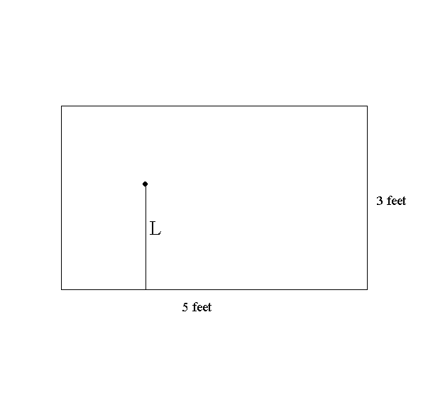
b) Find the probability that 1 <= L <= 2. Find the average probability density for L on the following intervals:
i) [1,2],
ii) [1,1.1]
iii) [.9, 1].
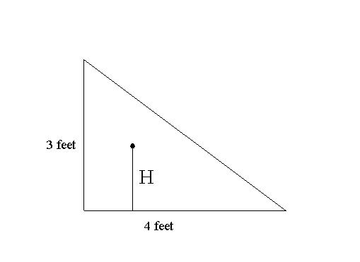
a) Let F(A) denote the probability that H < A where 0 < A < 3. Find F(1) , F(1.5) , F(2), and F(A). [Hint: For what region in the triangle will H<A?] Use a transformation figure and a graph to visualize F.
b) Find the probability that 1 < H < 2. Find the average probability density for H on the following intervals: i) [1,2], ii) [1,1.1] iii) [.9, 1].
In problems 6 through 10, suppose X is a random variable which takes values in the interval [0,2] and that F(A) gives the probability that X <= A where 0<A<2 . Use a transformation figure and a graph to visualize these functions.
a. Find the average probability density of X in the intervals [1,2], [1,1.1], [0,1], and [.9,1].
b. Find a number A where 0 < A < 2 where the probability that X < A is the same as the probability that A < X .
We allow a player to throw a dart 36 times and find the total score for the player as well as the average score (the total divided by 36). [The average will be a number between 5 and 55.] Give a total score and an average that you might expect for a player with no special skill. [These numbers might be called the expected score and the expected average for the game.] Discuss your reasoning and show your work leading to your proposed solution.
Suggestion: You might investigate the similar problem with 2 regions and 4 throws and then 4 regions and 16 throws as a way to begin thinking about the problem. How many darts do you think would fall in each region?
Extension: For each of the 36 throws, suppose we measure the
distance the dart lands from the center. What do you think the average
distance would be for a player with no special skills. Explain your reasoning,
any connections with the expected average score in the game, and whether
you have any belief about the accuracy of your response. (Is it an underestimate
or an overestimate?)