Preface: In section IV.B we saw many cases
where finding the solution of a differential equation involving core functions
was simple and direct. Unfortunately, solving differential equations is
not always so easy. Some differential equations with very simple expressions,
such as y' = sin(x2), do not have solutions that
can be expressed in elementary terms. To aid in solving more difficult
differential equations we'll extend our understanding in this section by
exploiting the geometric interpretation of the derivative as the slope
of the line tangent to the graph of a solution. Keep in mind: The
geometric interpretation of a function is a graph in the plane, so our
objective in this section is to see how a differential equation gives information
that helps us visualize the graph of a solution. The Tangent Field: The geometric
interpretation of a first order differential equation gives a relation
between the coordinates (x,y) of a point in the plane and the derivative
of a solution at that point. Interpret the derivative as the slope of a
tangent line at (x,y) to obtain a graphical representation
of a differential equation.
At various points in the plane draw short segments of lines whose slopes
are determined by the differential equation. These segments help visualize
the graphic qualities of the solutions. The plane, now sprinkled with line
segments, is described as a field of tangents, or a tangent [direction
or slope] field.We will see how to sketch these fields as we proceed
through some examples.
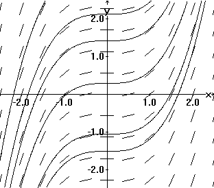
A tangent field determined by y' = x2
Solution curves drawn in a tangent field determined by y' = x2
But first let's think of drawing the graph of a solution to the differential
equation in the tangent field. Any tangents to a solution should have slopes
close to the slopes of nearby segments already drawn in the tangent field.
In this sense we can say that the shape of the graph of a solution fits
consistently with the line segments of the tangent field. This property
gives a method for sketching a solution's graph in a tangent field. Make
the solution curve's sketch fit with the segments as well as possible.
It's very much like the situation of children asked to connect dots to
discover a picture. The instruction now is to draw a curve starting at
some point (perhaps based on some initial condition) so that if the curve
passes through or near one of the line segments in the field, the tangent
to the curve should have a slope close to that of the line segment of the
field.
Integral Curves: Since the curves
drawn in the tangent field assemble information from the differential
equation and represent solutions to the differential equation, they are
called integral curves. Notice that the integral curves determined
by a differential equation of the form y' = dy/dx
= P(x) help visualize the indefinite integral $\int$
P(x) dx. The graphs represent members of the solution family by their
graphs.
Since a tangent field and integral curves for a differential equation
display only a sampling of the information contained in the differential
equation, these tools are most useful to suggest either results about a
particular solution to the differential equation or to give more qualitative
understanding about the general solution to the differential equation.
We'll illustrate the use of these tools first with some differentail equations
where we can find the solution. Then we'll turn to more chalenging examples
where a simple solution is not possible. To be more concrete, here's
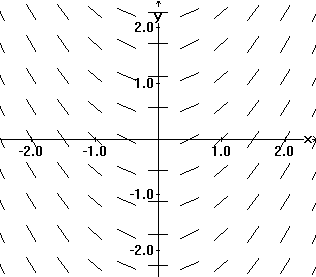
EXAMPLE IV.D.1: Draw segments of the tangent
lines at various points for the differential equation dy/dx = x
2, that is, draw a tangent field for dy/dx = x 2.
DISCUSSION:
x
y
dy/dx = x2
0
any
0
1
any
1
-1
any
1
1/2
any
1/4
-1/2
any
1/4
2
any
4
Figure IV.D.i
Figure IV.D.ii
Figure IV.D.iii
The chart in Figure IV.D.i shows that the x values have been
chosen (arbitrarily) to be 0, 1, -1, 1/2, -1/2, and 2. Because the derivative
here depends only on the first coordinate of a point, the y value
has not been specified. The segments of the tangent lines on the graph
have been drawn so that the midpoint of the segment is one of the points
with the chosen first coordinates. The resulting graph in Figure IV.D.ii
gives the appearance of several columns of parallel line segments. Each
column's segments have an appropriate slope to satisfy the differential
equation for the x value for that column.
To repeat the idea here, at selected points in the plane the tangent
field has a line segment with its slope determined by the differential
equation.
Now consider Figure IV.D.iii. This is a graph of some integral curves
for the differential equation dy/dx = x 2.
They are the graphs of y = (1/3) x 3 + C determined
by a few values of C.These curves are parallel in the sense that
the difference between Y values of any two of these curves is a constant.
This is consistent with the geometric
interpretation of Theorem 4.2. [The optical illusion that the curves
are further apart at the center of the figure and closer at the left or
right sides of this figure is a result of the tendency of the eye to relate
these curves by their closest points instead of vertically.]
More examples may help you understand the concept of a tangent field
and the visualization of integral curves-- so consider these:
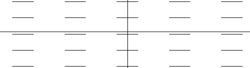
EXAMPLE IV.D.2. Graph the tangent field for y'= 0 .
Solution:
Figure IV.D.iv
Discussion: From the tangent field in Figure IV.D.iv
the integral curves for this tangent field would appear to be horizontal
lines. This agrees with our knowledge from Theorem
4.1. that the solutions to this differential equation are constant
functions.
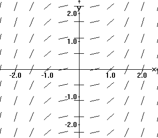
EXAMPLE IV.D.3. Graph the tangent field for y' = x .
Solution:
Figure IV.D.v
Discussion: Here again the tangent field graph in Figure IV.D.v
suggests the graphs of the solution integral curves will form a family
of parallel curves. It is fairly easy to draw tangent fields where the
derivative depends only on the first coordinate variable, x. For
x
= a, you need only compute dy/dx at that value of
x from the differential equation. Then you can draw in the figure
numerous line segments with slope dy/dx along the vertical
line X = a.
EXAMPLE IV.D.4. Graph the tangent field
for y' = x - y. Describe the graph of the
solution where y(0) = -1
Discussion: Here the problem is more subtle because the derivative
depends on both coordinates of the point. For example, at the point (-1,2)
we have that y' = -1 - 2 = -3 while at (0, -1) we find that y'
= 0 - -1 = 1. A first approach to this tangent field is to select several
points on the plane and compute y'. Figure IV.D.vi(a) shows an efficient
way to display this information in a table.
y/x
-2
-1
0
1
2
2
-4
-3
-2
-1
0
1
-3
-2
-1
0
1
0
-2
-1
0
1
2
-1
-1
0
1
2
3
-2
0
1
2
3
4
Figure IV.D.vi(a)
Figure IV.D.vi(b)
Figure IV.D.vi(c)
The entries in the table are the values of y' determined from the
x
value at the top of the column and the y value at the left of the
row. Thus the entry in the column with x = a and row with
y = b will be a-b. The tangent field is then drawn using
this information to plot the appropriate line segments as Figure IV.D.vi(b)
indicates.
After this kind of detailed work you may have noticed that for all points
on the line y = x, the value of y' is 0 . This can be seen
easily by noticing that y' = 0 implies that 0 = x - y. Similar
analysis shows that y' = 1 when 1 = x - y, that is along
the line y = x - 1. In general the same analysis shows that
y'
= m when m = x - y, that is along the line y = x - m. This
allows a more complete picture of the tangent field as drawn in Figure
IV.D.v(c). Notice that this figure suggests two essentially different types
of integral curves separated by the line y = x - 1. In fact
the line y = x - 1 is also an integral curve for this differential
equation since for any point on this line, 1 = y' = x - y.
Thus the solution with y(0) = -1 is given by this special solution
y = x - 1.
GeoGebra: Table with Tangent Field
Figure IV.D.vi(d)
Using SAGE to draw a Tangent Field:
Click on the Evaluate button.
You can change the function for the Tangent
Field
Problems IV.D
In problems 1-20, for each given differential equations (a) sketch the
tangent field showing tangents in all four quadrants. (b) Draw three integral
curves on your sketch including one through the point (1,2); (c)
Suppose that a solution to the differential equation has value
2 at 1. Based on your graph, estimate the value of that solution
at 2 and at 4. If the values of the solution are too large for x = 2
or x=4 to be estimated from your graph, discuss briefly why this is happenning
based on your sketch.
1. y' = x 3
2. y' = x - 1
3. f '(x) = .5 x
4. dy/dx = 1 - x
5. L'(t) = 1/t ... t $\ne $
0
6. L'(t)= 1/(1+t) ... t $\ne $-1
7. DP(t) = 1/(t 2+1)
8. dz/dx = x/(x 2 + 1)
9. y' = 2y
10. y' = -y
11. dy/dx = -2y + x
12. dy/dt = -2t + y
13. y' = 1/y ... y $\ne $ 0
14. z' = 2/(1+z) ... z $\ne $-1
15. y' = y 2
16. P'(t) = t 2 + (P(t)) 2
17. dy/dx = -x/y y $\ne $0
18. dy/dx = -y/x
19. dy/dt = 1/t 2 ... t $\ne $ 0
20. y' = 1 /(x 2+y 2)...(x,y) $\ne $
(0,0)
Since indefinite integrals are solutions to differential equations, tangent
fields can be used to help sketch the graph of an indefinite integral.
When possible this can be matched against the graph of the solution found
symbolically. It can also be compared with the qualitative information
about the graph of the solution that analysis of the first and second derivative
yield.
For each of the following indefinite integrals use the tangent field
to sketch the graph of three indefinite integrals. Discuss the general
features of this graph based on whatever else you can gather from the integrand.
a) $\int 3x^2 - 2x + 1$
b) $\int t \sqrt{1+t^2}dt$
c) $\int$ sin(x)
cos(x) dx
d) $\int$ (1- x2
)-1
dx
e) $\int$ sin(x2) dx
f) $\int$ exp
(-x2) dx
A differential equation determines another family of curves which is geometrically
significant. Members of this family meet integral curves at right angles.
For each of the following differential equations sketch the tangent field
and three integral curves. Draw three members of the family of curves perpendicular
to the integral curves on the same graph.
a) y' = 1/x ... $x \ne 0$
b) y' =
x
c) dy/dx = 1 + x2
If possible, match the following differential equations with the appropriate
sketch of its tangent field if sketched.
a) y'= x 2 - y2
b) y'= |x|.5
c) y'= y - x
d) yy'= 1 ..y$ \ne $ 0
e) y'= 1 - y
(a) - (f) For each of the contexts in problem 10 of IV.A draw a tangent
field for that sector of the plane which would be meaningful for the circumstances.
Match the following differential equations with the appropriate sketch
of its tangent field as drawn.
a) y'= cos(x)
b) y'= cos(x) + 1
c) y'= cos(x) - 1
d) y'= 2cos(x)
e) y'= .5 cos(x)