In the previous work using Maclaurin's polynomials, the focus of attention has been on estimating the values of a function f based on information developed when x=0. To find estimating polynomials P_n (x) for the function f expressed in powers of x we have calculated f(0), f '(0), f ''(0), and so on. For some functions it is impossible or at least inconvenient to find this information related to x = 0. However,often it is still  possible to evaluate a function and its derivatives at another point in the domain, say x = a. Taylor's theory can handle this additional generality quite easily based on our previous work at x=0. The main theorem of this chapter states the most general result, which we will refer to as Taylor's Theorem. Before stating and proving this theorem, we consider the Taylor polynomial for a `C^{oo}` function at x=a which generalizes the Maclaurin polynomial.

Definition IX.D.1: Suppose f is a `C^{oo}` function in an interval containing x = a. Let

`P_n(x;a,f(x))`  is called the Taylor polynomial of degree n for f at x=a.

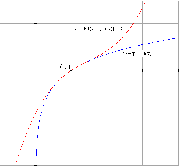
Example IX.D.1: Find `P_3(x;1,ln(x))`.

Solution: We compute the appropriate coefficients as follows:

`P_3(x;1,ln(x)) = 0 + 1(x-1) - 1/2(x-1)^2 + 2/6(x-1)^3 =(x-1) -{(x-1)^2}/2 + {(x-1)^3}/3 `.

Here is the graph of this polynomial compared to that of ln(x).

Note: The Taylor polynomial of f at x = 0 is the Maclaurin polynomial of the same degree for f, i.e.,

The next proposition shows how the Taylor polynomial generalizes the Maclaurin polynomial as the solution to a differential equation.

Proposition IX.D.1:
Suppose f is a `C^{oo}` function for an interval containing  `x = a` and let `p(x) = P_n(x;a, f(x))`.

Proof: This should be a fairly straight forward exercise.

Theorem IX.D.2:(Taylor's Theorem)  Suppose f is a `C^{oo}` function for an open interval I that contains `x = a`. For any `b` in I, `f(b)` is approximately equal to `Pn(b;a,f(x))`. Furthermore, if `R_n(b) = f(b) - P_n(b;a,f(x))` then there is a number `c` between `a` and `b` where

Proof: Consider `g(t) = f ( a + t )`. Essentially `g` shifts the information of the function  `f`. The function `g` has its values for points in an interval containing 0. Now apply the main proposition for Maclaurin's polynomials, Theorem IX.B.1, to `g`. Estimate the value of `g` at `x = b-a`. Thus when `b` is close to `a`, `b-a` is close to `0`, so

But `g(0) = f(a)`, `g'(0) = f '(a)` , ..., and `g^{(n)}(0) = f^{(n)}(a)` , so

We noted previously that `g(b-a) = f(a + b-a ) = f(b)`, so we have that `f(b)` is estimated by `P_n(b;a,f(x))`.

Now from IX.B.1 there will be a number `q` between `0`and `b-a` so that the difference between `g(b-a)` and `P_n(b-a,g(x))` is equal to

But if we let `c= a+q`, then we have immediately that `c` is between `a` and `b` and

EOP

Example IX.D.1: (Continued) We use `P_3(x;1,ln(x))`  to estimate `ln(1.1)` and `ln(.9)`. Since the expression for `P_3(x;1,ln(x))` involves powers of `x-1`, first note that when `x = 1.1`, `x-1=.1` so we have that

Exercises:
In problems 1-10 for the indicated function f  find the Taylor polynomial P _n(x;a, f(x)) of degree n about x = a. On the same axes, graph f (x) and  P _n(x;a, f(x)).

1. f (x) = 1/x ; n = 4; x = 1.
2. f (x) = 1/x ; n = 4; x = 2.
3. `f(x) = sqrt (x)` ; n = 4; x = 1.
4. `f(x) = sqrt (x)` ; n = 4; x = 4.
5. `f(x) = root (3) (x)`; n = 4; x = 1.
6. f (x) = 1/x² ; n = 4; x = 1.
7. f (x) = 3 + 5x + 3x² + 4x³ +  x⁴; n = 2, n = 3, n = 4; x = 1.
8. f (x) = 1/x ; n = 4; x = a>0.
9. `f(x) = sqrt (x)`; n = 4; x = a>0.
10. f (x) = ln(x) ; n = 6; x = 1.
11. f (x) = ln(x) ; n = 6; x = a>0.
12. Use problems 1 and 2 to estimate 2/3 = 1/(3/2). Compare the results and the related remainder terms.
13. Use problems 3 and 4 to estimate `f(2) = sqrt (2)`  and `f(3) = sqrt (3)` . Compare the results and the related remainder terms.
14. Use problem 10 to estimate `ln(1.1), ln(.9), ln(.8)`, and `ln(1.2)`. Discuss the error in each estimate.
15. Use the properties of logarithms and the previous problem to estimate `ln(2) = ln( 1.44/.72 )`.
16. Use the properties of logarithms and the previous problems to estimate ` ln(5) = ln( 4 /.8)`.
17. Use the properties of logarithms and the previous problems to estimate `ln(9) = ln(10 * .9 )` and then `ln(3)`.
18. Using the Taylor polynomial of degree 6 for ` ln(x)` at x=1, estimate the area of the region enclosed by the graph of `y= ln(x)`, x = 1 and x = 2. Discuss the error in this estimate based on the Taylor remainder formula. Compare this estimate to the estimate for the same area based on Simpson's method with n = 6.