Chapter V. E. Riemann Sums and Definition of the Definite Integral.  [Draft in Progress.]

© 2014 M. Flashman

In the previous sections of this chapter we have used a rather simple definition of the definite integral based on Euler Sums. The interpretation of these sums in Chapter V.A related these sums to finding areas, determining the net change in position of a moving object, or looking at the change in the second coordinate for an integral curve over an interval. In our examination of other methods for estimating the definite integral for a continuous function over a compact interval, we used accumulated information about the function at points selected either for the ease with which they designated (endpoints and midpoints) or their relation to function's values on the interval (maximum and minimum). The two general principles for these estimates was what was good for one would be good for all, and the more the merrier. Following these principles when partitioning an interval we made the length of the subintervals all equal.
For the interval [a,b], we made N subintervals of length $h = \Delta x = \frac {b-a} n$ and the resulting partition $\mathcal P$ = { $a = x_0, x_1, x_2, ..., x_{n-1}, x_n = b$ } would use points  $ x_k = a + k \cdot \Delta x$.

In this section we will examine a more general approach to describing the definite integral of a function called the Riemann integral, usually attributed to Bernard Riemann (1826-1866). The definite integral based on the Euler sums is just a special case of the more general Riemann sums. Every continuous function will have a Riemann integral for a compact interval, so the computational results we have obtained for continuous functions using the Euler sums will not change for this extension. However, although every function that is Riemann integrable will be Euler integrable, there are functions (non-continuous) which have an Euler integral but do not have a Riemann integral.

Extended Euler: Before proceeding to the general Riemann sums, we'll extend the description of Euler sums for a function P on the compact interval $[a,b]$ in a way that will include the right hand endpoint and midpoint estimates. For N a positive integer, as usual we let $h = \Delta x = \frac {b-a} n$ and $x_k = a + k \cdot \Delta x$  for $k = 0, 1, 2, ..., N$.  Now choose numbers $w_k$ so that $x_{k-1} \le  w_k \le  x_k ; k = 1$ to $N$  and let $\mathcal W= \{ w_1, w_2, ... ,w_{n-1}, w_n \}$. These numbers might be midpoints, endpoints, or extreme points for P. What is sampled in one subinterval does not effect what is chosen in another. The choice of a $w_k$ is arbitrary. Only in a very limited sense have we followed the principle of what is good for one is good for all. [In fact if we want to be very clever for a continuous function we would choose $w_k$ so that $P(w_k) \cdot \Delta x = \int_{x_{k-1}}^{x_k} P(x) dx$ where the integral here is the Euler integral.] Now we form the extended Euler sum, $S(P,N,\mathcal W) \equiv \sum_{k=1}^N P(w_k) \Delta x $. We still employ the principle of the more the merrier to make better estimates and we can define the extended Euler definite integral as follows:

Definition V.E.1. Suppose there is a number $I$ so that as $N \rightarrow \infty$ with any choices of  $\mathcal W$, the sums $S(P,N,\mathcal W) \rightarrow I$, then $I$ is called the (extended Euler) definite integral of $P$ over the interval $[a,b]$. With the notation of limits and integrals we have

           $I  \equiv \int _a^b P  \equiv  \int _a^b P(x) dx  \equiv  \stackrel {\lim}{_{N  \rightarrow  \infty}} S(P,N,\mathcal W) =    \stackrel {\lim}{_{N  \rightarrow  \infty}} \sum_{k=1}^N P(w_k) \Delta x$ .

 Comments: 1. Since we can let $w_k=x_{k-1}$ for $k = 1$ to $N$, an Euler sum is one of the extended Euler sums, and thus for any function which has an extended Euler integral, the extended Euler integral is the Euler integral. Since it can be shown that any continuous function has an extended Euler integral, we use the same integral notation for the extended Euler integral, namely $I  \equiv  \int _a^b P(x) dx $.
      See problem *** for an example of a (non-continuous) function which has an Euler integral but does not have an extended Euler integral.

2. The right hand endpoint estimates for the Euler integral are extended Euler sums with $w_k = x_k$ .The midpoint estimates for the Euler integral are extended Euler sums with $w_k = m_k =  \frac{x_k + x_{k-1}}2$.

3. Interpretations of the extended Euler integral match the interpretations of the Euler integral. For estimating area, changes in position, or integral curves, the extended Euler allows more flexibility in the choice of numbers at which to evaluate the function $P$ as a sampling of what is happening with the height of the approximating rectangles, the velocity estimate for the moving object, or the slope of the approximating line segment in each subinterval.

4. At this stage you might ask, "Why use an extended Euler sum to estimate the definite integral?"

The following example illustrates that sometimes it is more convenient to choose values of the function $P$ without having to use any specified procedure to make a quick estimate of an integral.

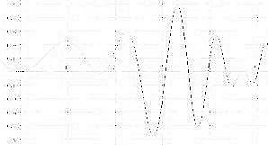
Figure 1

Interval wk P(wk) [1,2] w1 0.2 [2,3] w2 -0.1 [3,4] w3 0.1 [4,5] w4 0.05

Example V.E.1: The graph of P is given in figure ***. Using $N = 4$ and an extended euler sum we can estimate the definite integral of $P$ over $[1,5]$, i.e., $\int _1^5 P(x) dx$. Rather than choose numbers based on a fixed procedure as we might for an euler sum estimate, we can make a much better estimate by looking at the four sub-intervals and selecting a value of P for some point in that interval in a way that gives a rectangle of area that approximates the definite integral determined by P for that sub-interval. The following table records these choices. Notice that we do not record the actual numbers w₁, w₂, w₃, and w₄ since we only need the values of P at these points which we can estimate from the graph. Since Δx=1 for this partition, we make our extended Euler sum estimate for the integral as .2 + -.1 + .1 + .05 = .25 . Notice that a left hand endpoint Euler estimate would be about .6 for the same graph, a right hand estimate would be about .2, a trapezoid estimate would be about .4, a midpoint estimate would be about -.1, and the Simpson's estimate would be about 0.07. An estimate of the actual integral was determined using technology to be about .20.

Riemann Sums : One of the more inefficient aspects of the Euler integrals is the reliance on a partition of the interval into segments of equal length. Though this may seem an efficient and fair way to make a sampling of values of the function P, it fails to take advantage of functions that are almost constant for a long interval and then vary considerably over a shorter interval. An Euler sum approach makes many measurements on the longer interval where a few would suffice while making a few if any measurements on an interval where the variation in the function's value might effect greatly the final estimate .

It's like the story of the hare and the tortoise. If we observe the tortoise we don't need many observations to estimate how far the tortoise will go in a fixed amount of time. But observing the hare is very different. Certainly while the hare is resting most of the time the tortoise is plodding along, but if that's the bulk of our sampling we may miss those very brief moments, when the hare turns on its speed. We would never expect that the hare travels almost the same distance as the tortoise for the same overall time interval and that at the end the race is very close, even if the tortoise does win. Certainly we need a different approach to observing the hare if we are going to predict the hare's position with the same number of observations of velocity as we make of the tortoise.

The Riemann sum approach allows more flexibility and choice to estimating the definite integral. It adds the ability to freely choose the lengths of the individual subintervals. To do this we change the organization of our computations. We begin not by selecting a  value for $N$ and finding $\Delta x$, but instead by choosing the partition of the interval $[a,b]$. In other words we start with $N-1$  numbers between $a$ and $b$, denoted with $x$'s and subscripts, $a = x_0 \le x_1 \le x_2 \le... \le x_{N-1} \le x_N = b$ , which as a set is denoted by $\mathcal P$. Notice that by allowing some of these numbers to be equal we don't even care that some may be repeated . [Of course, these numbers could be the same numbers used for an Euler sum, but they don't have to be... so the Riemann approach has allowed for many more possibilities.] Now the partition $\mathcal P$ results in $N$ subintervals, $V_k =[x_{k-1}, x_k]$, for $k =1, 2,, ..., N$ determined by the partition numbers $x_k$. We denote those lengths of these subintervals by $\Delta x_1 \equiv x_1-x_0, \Delta x_2 \equiv x_2-x_1$, and in general, $\Delta x_k \equiv x_k - x_{k-1}$ for $k =1, 2,, ..., N$. As with the extended Euler sum, we choose sampling  numbers $w_k$ in the subintervals, $V_k$  for evaluating the function,
$x_0 \le  w_1 \le  x_1 \le  w_2 \le  x_ 2 \le  w_3 \le  x_3 ... \le  w_{N-1} \le  x_{N-1} \le  w_N \le  x_N$.  More notation as we let $\mathcal W = \{ w_1, w_2, ... ,w_{N-1}, w_N \}$.

With all the choices made and notation established we can now define the Riemann sum  $RS(P, \mathcal P, \mathcal W)$ for this partition $\mathcal P$ and the number choices $\mathcal W$. 

Note: A midpoint estimate with N=3 gives a slightly more accurate result with less computation.  Can you explain this?
Draw a sketch of the graph and consider the concavity on the intervals.

Without Limits (Darboux?):

                $M_k ≡ sup \{ f(x): x_{k-1} \le  x \le  x_k \}$ [maximum when $f$ is continuous]

                $m_k ≡ inf  \{ f(x): x_{k-1} \le  x \le  x_k \}$ [minimum when $f$ is continuous]

               $L_P \equiv \sum_{k=1}^{k=n} m_k  \Delta x_k$ [The Lower Riemann Sum]

[Continuous Functions are integrable]