We have already explored one model for learning in which the learning rate was a positive decreasing function of time, i.e. $ L'(t) = \frac 1t$. The solution to this model with the initial condition $L(1) = 0$ led us to the natural logarithm and a model for learning that had the values of $L(t)$ unbounded in the sense that for any number $B$ there was some $t$ where $L(t) > B$. Although this model is very encouraging in terms of the unbounded increase in learning, it does not match very well with much experience. In many situations there are bounds to what can be learned no matter how much time is spent in the process. In trying to find a model for such a learning curve, we examine a similar rate of learning that is positive but less than $\frac 1t$.

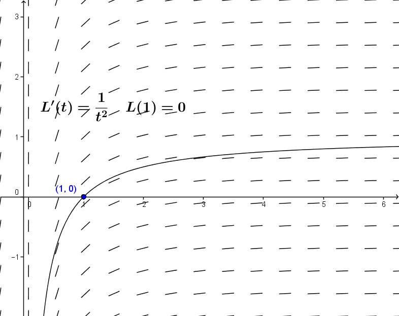
Example VI.D. 1. Suppose $L_2'(t)= \frac 1{t^2}$ and $L(1) = 0$. Find $L_2(2)$ and discuss the value of $L_2(t)$ when $t > > 0$.

Solution: This problem is not too hard since $G(t) = \frac {-1}t$ has $G'(t)= \frac 1{t^2}$. Thus $L_2(t) = \frac{-1}t + C$. Solving for $C$ we use $0 = L_2(1) = -1 + C$ so $C = 1$ and $L_2(t) = 1 - \frac 1t$ for all $t > 0$.
To respond to the problem, we have $L_2(2) = 1 - \frac12 = \frac 12$ .When $t > > 0$ then $L_2(t)$ is close to $1$.
Comment: We now have a model for learning with bounded growth. At this stage we'll modify the differential equation just slightly and consider the same questions for a derivative function for which we do not yet have an antiderivative.

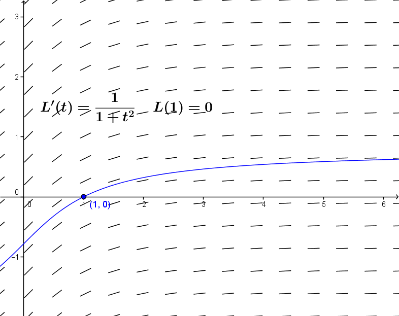
Solution: At this stage we have no elementary function which has  $\frac 1{1+t^2}$ for its derivative.
Looking at the tangent field and a sketch of the integral curve for this differential equation gives some idea of the shape of the solution. [See Figure VI.D.2]

We consider $A'(t)$ and $L_2'(t)$ as the rates at which the amount learned is changing.
Then since $\frac 1{1 + t^2} < \frac 1{t^2}$ for any $t > 1$, the amount learned at any time $t$ according to the $L_2(t)$ model is larger than that learned according to the $A(t)$ model. [See Figure VI.D.3.]

$A(t)$ is increasing for all $t$, yet since $0 = A(1) = L_2(1)$ and  as $t$ gets large, $L_2(t) \rightarrow 1$, it must be that $A(t) < L_2(t) < 1$ for all $t$ .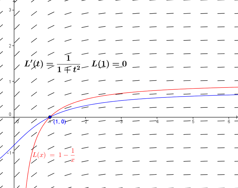

By careful analysis of this situation it should seem reasonable that as $t$ gets large, $A(t)$ approaches some specific number that is at most $1$.
Later this section we will see what this number is, but for now we continue our analysis to try to find $A(2)$.
 

First, as we did with the model for L(t), we can estimate A(2) using Euler's method.[Can you explain why this is an overestimate?]
 

This is easy enough in theory because of the fundamental theorem of calculus, but it doesn't express the funtion A as any elementary function that we have studied yet in the calculus.

To develop this differential equation further we introduce a slight variation on the function A, changing the initial condition of the differential equation to arrive at a more enlightening solution.

Suppose A ₀'(t) = 1/(1+t ²) and A ₀(0) = 0. Then since A'(t) = A ₀'(t) for all t, A(t) = A ₀(t) + C for some constant C. We'll come back to A(t) later in this section, but now we'll focus on A ₀.

To understand A ₀, we look at F(x) º A ₀( tan(x)). Using the chain rule and the derivative of the tangent function together with the differential equation defining A ₀ we have that

Now this means that for all x in (-pi /2,pi /2), F(x) = x + K for some constant K. Evaluating F at 0, we see that   F(0) = A ₀( tan(0)) = A ₀(0) = 0 = 0 + K,  so F(x)= x for all x in (-pi /2,pi /2). This means that for these value of x, A ₀(tan(x)) = x

But the function that satisfies this property is the arctangent function.
Thus A ₀(t) = arctan(t) for all t.
This result can be expressed in a more direct fashion, namely, arctan'(t) = 1/(1+t ²).

Example VI.D.2 (continued) From the last result we have that A(t) = arctan(t) + C and therefore
0 = A(1) = arctan(1) + C = pi /4 + C. So C = -pi /4 and A(t) = arctan(t) - pi /4.

Recalling the basic properties of the arctangent function allows us to answer the original questions about A.

A(2) = arctan(2)-pi /4 which is about  0.32175, and

Derivatives of Inverse Trigonometric Functions.

At this point we'll stop a moment to give a more geometric justification of the result on the derivative of the arctangent. We'll use the same technique to find the derivative of the arcsine function, leaving the derivatives of the arccosine and the arcsecant as exercises.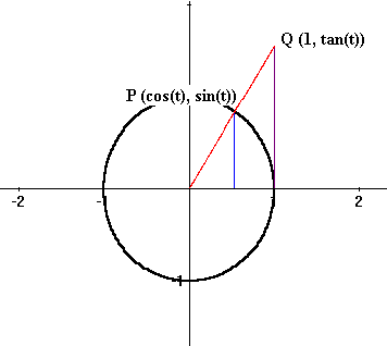

Theorem VI.D.1: For all x , arctan'(x) = 1/(1 + x ²).

Proof: Recall that tan'(t)=sec ²(t) for all t in (-pi /2,pi /2).

Recall also that the tangent function can be visualized by drawing an arc of length t on a unit circle to determine the point P with coordinates (cos(t), sin(t)), drawing the radius through P to meet the tangent line to the circle X=1 at the point Q with coordinates (1,tan(t)). [See Figure VI.D.4.]

Now a change of angle, dt, gives a corresponding change in the position of Q, called dy where y=tan(t) . Then the ratio dy/dt is approximately sec ²(t) so the ratio of dt/dy is approximately 1/sec ²(t). But t is the arctan(y). Now when dy -> 0,

dt/dy -> 1/sec ²(t), so we have arctan'(y) = 1/sec ²(t) = 1/(1+tan ²(t)) = 1/(1 + y ²).

Changing the name of the variable completes the argument. EOP

Corollary VI.D.2:.

We now turn our attention to the inverse function of the sine, called the arcsine.

Theorem VI.D.3: For x with -1 < x < 1 , arcsin'(x) = 1 / sqrt (1-x ²).
Proof: Recall that sin'(t) = cos(t) for all t in (-pi /2,pi /2)
.
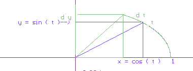
The sine function can be visualized [See Figure VI.D.5.] by drawing an arc of length t on a unit circle to determine the point P with coordinates (cos(t), sin(t)), then drawing the horizontal line through P to meet the vertical axis at the point S with coordinates (0,sin(t)).

Now a change of angle, dt, gives a corresponding change in the position of S, called dy where y=sin(t). Then the ratio dy/dt is approximately cos(t) so the ratio of dt/dy is approximately 1/cos(t). But t is the arcsin(y) so when dy -> 0, dt/dy -> 1/cos(t). Thus we have

Changing the name of the variable completes the argument. EOP

Corollary VI.D.4:  .
Theorem VI.D.5: For x with -1 < x < 1 , arccos'(x) = -1 / sqrt (1-x ²).

Proof: Though a detailed proof of this result can be obtained using the derivative of the cosine (see exercise 19), the fact is most easily understood by noting that arccos(x) = p /2 - arcsin(x). EOP.

Theorem VI.D.5: For x with 1 < x or x < -1 ,  arcsec'(x) = 1/[ x sqrt(x ² - 1)].

Proof: Left as an exercise.

Comments: The derivatives of functions involving the inverse trigonometric functions are found using rules for differentiation examined previously in Chapter III. Applications of these functions arise in situations where angle measurement can be used to control some other measurement. What is somewhat more difficult is recognizing these functions in integration problems. Unlike differentiation, there are no completely general methods for attacking integration. We will explore some further integration methods later, but for now here are two examples showing how substitution can come into play to find integrals related to the arctangent.
 
 

Example VI.D.iii. Find a)and b).

Solution: a) Let u = exp(x) so that du = exp(x) dx and this integral becomes

.

b) Let u = 1 + x, so that du = dx and this integral becomes

.

Comment: Integrals related to the arcsine function also can be complicated by substitutions and the need to recognize an appropriate choice for the substitution. In b) this meant supposing that 2 + 2x + x ² = 1 + u ². Solving for u we now have u ² = 1 + 2x + x ² = (1 + x) ² so u = 1 + x and we can continue.

Exercises VI.D

Find derivatives for the following functions:
 

1. f(x) = arctan (5x)
2. y = tan ^-1 (x ³)
3. g(t) = arctan(e ^x)
4. s(u) = 1/arctan(u)
5. f(x) = arcsin (5x)
6. y = sin ^-1 (x ³)
7. g(t) = arcsin(e ^x)
8. s(u) = 1/arcsin(u)

Find the following integrals:
9. 
10. 
11. 
12. 
13. 
14. 
15. 
16. 
17. 
18. 
19. Give a proof of the derivative formula for arccos(x) using the unit circle and the derivative of the cosine.
20. Give a proof of the derivative formula for arcsec(x) using the unit circle and the derivative of the secant.
21. Approximate = p using any of the methods for approximating the definite integral. Explain your result.
22. If y = arctan(x) then by definition tan(y) = x. Use implicit differentiation with this fact to show arctan'(x) = 1/(1 + x ²).
23. If y = arcsin(x) then by definition sin(y) = x. Use implicit differentiation with this fact to show arcsin'(x) = 1/ sqrt (1 - x ²).
24. If y = arcsec(x) then by definition sec(y) = x. Use implicit differentiation with this fact to show arcsec'(x) = 1/[x sqrt (x ² - 1)].

 

 
 
 
 
 
 
 
 
 
 
 
 
 

There are many more possible models for learning that involve positive, decreasing functions. For problems 25-30 assume that L'(t) = P(t) and L(1) = 0.

1. Give an exact answer or an estimate for L(2).
2. Discuss briefly the convergence question for t>>0.
3. When possible, estimate the limit of L(t) as t -> infinity.
25. P(t) = 1/t ³
26. P(t) = 1/t ^3/2
27. P(t) = e ^-t
28. P(t) = 1/(t ² + 6t + 10)
29. P(t) = 1/(t ³ + 1)
30. P(t) = exp(-t ²)