IV.H. The Fundamental Theorem of Calculus: A Differential Equations Approach. [Draft - in progress]
© 2000 M. Flashman
 
  Preface: In the IV.G we solved the differential equation s'(t) =1/(t+1), with initial condition s(0) = 0. Our solution used the function F(t) defined as the area of a related planar region controlled in size by t. That example generalizes without much difficulty to a key result about the ability to solve differential equations of the type S'(t) = P(t). In the generalization P(t) must be sufficiently like 1/(t+1) to allow the same kind of argument we gave in IV.G for its justification. Looking back over the discussion in IV.G  you should notice that two facts were crucial elements of the argument:
(1) 1/(t+1) > 0 for t > 0,and
(2) 1/(t+1) is a continuous function for t > 0 .
We used (1) and (2) subtly. In our graphical definition of F these conditions ensured that the region in the plane had an "area". The continuity of 1/(t+1) was used in two other ways. It allowed us to find bounds on the value of the expression F(a+h) -F(a) [ by applying the Extreme Value Theorem] and to find the limit of 1/(a+h+1) as h -> 0. 
Though we will see in Chapter V that the result of IV.G can be generalized even further, we state here our main result in a slightly restricted form. We describe this theorem as "fundamental" because of the general and deep nature of its conclusion.  Recall that we discussed at the beginning of this chapter that given a positive continuous function representing the velocity of a moving object, it is always possible determine the position of the object during its trip, i.e., a position function depending on time that changes at the specified velocity. The theorem gives a geometric version of this trip story.
Preview to generalizing in Chapter V: We generalized the tangent line slope, the marginal cost, and the instantaneous velocity concepts in Chapter I to develop the concept of the derivative of a function.This was first conceived of as a number and then developed further to the derivative function. Similarly in Chapter V we will generalize the estimations used in the changing position, marginal costs, and area contexts to develop a number called the definite integral of a function over an interval and the related function family of the indefinite integral. 
We found that, like velocity, the derivative had important functional features. Similarly, like area and position, the definite and indefinite integrals have very useful numerical and functional features for analyzing and solving differential equations and many other applications.


Theorem IV.4 The Fundamental Theorem of Calculus For Differential Equations (first draft). 
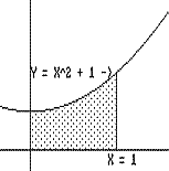
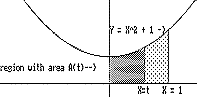
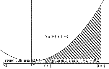
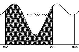
[See Figure IV.H.i.] 
If P is a positive continuous function on [A,B], then there is a function F with F'(t) = P(t) for all t where A<t<B
In fact, F can be defined at x = t to be the area of the region enclosed by the X -axis, the line X=A, the line X=t, and the graph of the function P, i.e., Y = P(X)[1]
  
Figure IV.H.i
Comment: At this stage the details of the proof of Theorem IV.4 are not essential. The proof, given in IV.H Appendix, follows the general outline of the argument of Example IV.G.3. In our discussion so far we have used the notion of area of a planar region in an informal and intuitive sense. In Chapter V we will generalize our experience with area and Euler's method. This will give a more firm foundation to our use of area as an interpretation. A more general formulation will also allow other interpretations to take advantage of the mathematical results expressed in the Fundamental Theorems of Calculus as presented in Theorems IV.3 and IV.4
 

Now we will look at a simple but important example showing the application of the Theorem IV.4 to find area. You should compare this and the next example with Example IV.F.4 which used Theorem IV.3 (the evaluation form of the Fundamental Theorem of Calculus) to find the area.
 
Example IV.H.1. Find the area of the region enclosed by the X- axis, the Y- axis, the line X=1, and the graph of the function Y = X 2 + 1. [See Figure IV.H.ii]. 

Solution: Let A(t) be the area of the region enclosed by the X-axis, the Y-axis, the line X = t, and the graph of the function Y = X 2 + 1.  The problem can be restated more simply now: Find A(1). [See Figure IV.H.iii.] The Fundamental Theorem (first draft) applies to say that  A'(t) = t 2 + 1 with A(0) = 0.  This differential equation with initial condition has a unique solution, namely,  A(t) = t 3/3 + t 
Therefore the area of the region is A(1) = 13 / 3 + 1 = 4/3. 

Solution: Let A(t) be the area of the region enclosed by the X -axis, the Y -axis, the line X=t, and the graph of the function Y = X 2 +1. The problem is to find A(1). [See Figure IV.H.iii.] The Fundamental Theorem (first draft) applies to say that A'(t) = t 2 + 1 with A(0) = 0. This differential equation with initial condition has a unique solution, namely, Therefore the area of the region is A(1) = 13 /3 + 1 = 4/3. 

Follow  up:  Notice that if the problem had used X = 5 instead of X = 1 for the right hand boundary of the region, the solution would have needed A(5) instead of A(1).  Thus the area of the region enclosed by the X-axis, the Y- axis, the line X = 5, and the graph of the function Y = X 2 + 1  is 

 A(5) = 5 3/3 + 5 = 125/3 + 5 = 140/3 = 46 2/3. 
  
Figure IV.H.ii  
  
Figure IV.H.iii

Example IV.H.2: Find the area of the region enclosed by the X -axis, the lines X=1, X=5 and the graph of the function Y = X 2 + 1. [See Figure IV.H.iv.] 
We'll present two solutions to this problem using Theorem 4.4. 

Solution 1: An examination of Figure IV.H.iv should help in analyzing the problem. 
Let B be the area of the region in question. Then we see that the region in this example joined to the region of Example IV.H.1. forms the region enclosed by the X -axis, the Y-axis, the line X=5, and the graph of the function Y=X 2 + 1. Using the notation of the previous problem and its follow up together with the additive property of area, we have that A(1) + B = A(5). 
  Thus B = A(5) - A(1) = 140/3 - 4/3 = 136/3 = 45 1/3. 

Solution 2: For this solution, let B(t) denote the area of the region enclosed by the X-axis, the lines X=1, X=t, and the graph of the function Y = X 2 + 1. [Figure IV.H.v.] Then B(1) = 0 and by the Fundamental Theorem of Calculus B'(t) = t 2 + 1. We solve this differential equation so that B(t) = t 2/3 + t + C. 
Using B(1) = 0 we solve for C, so that B(t) = t 2/3 + t - 4/3. 
Now the problem reduces to finding 

B(5) = 5 2/3 + 5 - 4/3 = 45 1/3. 
 
 
Figure IV.H.iv 


Figure IV.H.v 

Comments: 1. The approach to area problems discussed in Theorem IV.3 and that used in the first solution to this example are not unrelated. In the end each approach used the difference of the values of a solution to the differential equation to determine the area. We will discuss these two results again in Chapter V, but for now we note that one method used approximations to make the connection between area and solving differential equations while the other ties them together with the geometry of area and the definition of the derivative.
 

2. Existence and Uniqueness. Theorem IV.4 states that when P is a positive continuous function then the differential equation S'(t) = P(t) has a solution. This result is described as an "existence" result since it declares that a solution to the differential equation does exist. After the work with tangent fields, Euler's method, and the heuristic arguments about the trip, the result should not come as a surprise. It and its generalizations are important because they allow us discuss solutions even when they have no simple description as elementary functions. Theorem 4.3 has a quite different message, building on the ability to solve the differential equation S'(t) = P(t). It declares that solving the differential equation and computing the net change S(b)- S(a) can be interpreted in other contexts, like area, where measurement can be estimated in a systematic way using sums of the form  P(x0). h + P(x1). h + P(x2). h +...+ P(x n-1). h.
We can rephrase this result with a focus on the value S(b). It says that value of a solution to the differential equation at b is completely determined by the value at a, S(a) and function P. In other words a solution to the differential equation S'(t)=P(t) is determined uniquely by the equation and an initial or bounday condition. It is in this way that Theorem 4.3 is considered a "uniqueness" result. 


Problems. In problems 1 through 6, use the Fundamental Theorem of Calculus to find the area of the region enclosed by the X-axis, the Y- axis, the line X=1, and the graph of the function .
  1.  y = x 3
  2.  y = x 2
  3. y = x 2 + x
  4. y = 16 - x 2
  5. y = x 5
  6. y = x n
  7. For the functions in problems 7 through 12, use the Fundamental Theorem of Calculus to find the area of the region enclosed by the X-axis, the lines X = 1, X = 3 and the graph of the function.

  8. y = x 3
  9. y = x 2
  10. y = x 2 + x
  11. y = 16 - x 2
  12. y = x 5
  13. y = x n
  14. Find the area of the region enclosed by the X-axis, X = p /2 and the graph of Y = sin(x).
  15. Find the area of the region enclosed by the X-axis, and the graph of Y = sin(x) for the interval [0, p].
  16. Find the value of t so that the area of the region enclosed by the X -axis, the Y -axis, the line X = t, and the graph of Y = X 3 is 4.
  17. Suppose that F is any function with F'(t) = t 2 + 1. Show that the area of the region enclosed by the X -axis, the lines X = 1, X = 5 and the graph of the function Y = X 2 + 1 is  F(5) - F(1).
  18. Suppose is a solution to the initial value problem, g'(x) = sin(x2 ) + 2 with f (0) = 0.
    1. Write a short exposition based on the work in chapter IV on this function. Include in your essay a disussion  of the various ways to visualize and estimate the values of g.
    2. Suppose is a solution to the differential equation f ' (x) = sin(x2 ). Give an equation relating  to the function g in part a. [Hint: What can you say about the difference g(x) - f(x).
     
  19. Consider Q(t) = -1 - t 2. Since Q(t)  < 0 for all t, Theorem IV.4 does not apply to this function, but it does apply P(t) = -Q(t) = 1 + t 2. Draw a figure to illustrate the following statements applied to P and Q:

  20. If Q is a negative continuous function on [A,B], then there is a function G with G'(t) = Q(t) for all t where A<t<B. In fact, G can be defined at x = t to be the opposite of the area of the region enclosed by the X -axis, the line X=A, the line X=t, and the graph of the function Q, i.e., Y = Q(X). The function G is the opposite of the function F defined in Theorem IV.4 for the function P(t) = - Q(t).
  21. Suppose A(x) solves the differential equation A'(x) = (1 + x2 ) -1  and A(0) = 0. Draw a figure that illustrates A(t) as an area of a region in the plane for t > 0.

[1] In fact this result can also be interpreted geometrically. It says that the slope of the tangent line to the graph of the area function F at the point (t, F(t)) is precisely the value of the function P(t). This connects this form of the Fundamental Theorem to Barrow's Theorem in Chapter 0.