ATM
¤

April 11, 2017
Complex Variables: Mapping Diagrams for 
Visualizing Complex Arithmetic and Functions
Dynamically with GeoGebra

Part I
Mapping Diagrams for Real Functions
Complex Arithmetic
Part II
Complex Functions


Martin Flashman
Professor of Mathematics
Humboldt State University


http://flashman.neocities.org/Presentations/MD.Reed.CV.9_19_16.html


3.1. Complex Functions ¤
Functions of complex variables can be visualized in a 3 dimensional figure by mapping diagrams between parallel complex planes.
Here are some examples of
linear functions, linear fractional (Moebius), and power functions I have built using GeoGebra .

3.1.1 A complex linear function can be visualized as a mapping from $\mathbb{C}$ to $\mathbb{C}$.    ¤
Example 3.1.1.1Mapping Diagram for Complex Linear Function from a Table (using points on a lattice for sampled domain.)
This example shows a linear function $f(z) = a + bz$ where $a$ and $b \in \mathbb{C}$
Move $a$ and $b$ in the plane to change the value of these complex number parameters.Move the "lattice" point in the plane to change the position of the lattice being used for the data in the table and on the mapping diagram.


Example 3.1.1.2 Mapping Diagram for Complex Linear Function (using points on circles for sampled domain.) 
¤
This example shows a linear function $f(z) = a + bz$ where $a$ and $b \in \mathbb{C}$ on a single complex number $z$ and points on a circle in the domain complex plane.
 

Use the "r" slider to change the radius of the circle in the domain for the mapping diagram.
Move $a$ and $b$ in the plane to change the value of these complex number parameters.
Notes:
  1. When $a=0$ and $b \in \mathbb{R}$ then $f$ is a dilation and the arrows lie on a section of a cone. The vertex of the cone is the focus point with axis orthogonal to the complex planes at $0$.
  2. When $a=0$ and $b = e^{i\theta} $ then $f$ is a rotation isometry about 0 by $\theta$ radians and the arrows lie on a section of an hyperboloid of one sheet between circles of equal radii centered at $0$.
  3. When $b = 1$ then $f$ is a translation isometry by $a$ and the arrows lie on a cylinder between circles of equal radii, one on the source centered at the $0$ and the other on the target centered at $a$.
  4. In general one can understand $f$ as a composition of these three types of functions, $f = s_a \circ r_{Arg(b)} \circ m_{|b|}$ where $m_{|b|}(z) = |b|z$ , $r_{Arg(b)}(z) = e^{Arg(b) i} z$, and $s_a(z) = a + z$.


3.1.2 Linear Functions visualized with cones and curves.  ¤
In the following figure for $f(z) = bz$ the mapping diagram is based on the cone for
$m_{|b|}(z) = |b|z$ as visualized in the previous figure. You can choose either the arrow mapping diagram or a mapping diagram using curves between $z$ and $f(z)$ on the cone to visualize $f$.


4.1 Visualizing Complex Linear Fractional Transformations [Moebius Functions] with Mapping Diagrams ¤
This example shows a moebius linear fractional function $$f(z) = \frac {a + bz}{c+z}$$ where $a$, $b$ and $c \in \mathbb{C}$ on a single complex number $z$. You can move $a,b$,and $c$ in the Graphics window to change the complex parameters for the Moebius function.


The sliders adjust the slope of the lines through $0$ and the radius of the circles centered at $0$ for the mapping diagram arrow source.
Notes:
  1. When $b=c=0$ and $b=1$ then $f$ is complex inversion and the circular based arrows cross on a line above the real axis.
  2. When $a=1$ and $c=0 $ then $f$ is the composition of complex inversion followed by translation by the complex number $b$.
  3. When $a=1$ and $b=0$ then $f$ is a translation isometry by $c$, followed by complex inversion.

4.2 Visualizing Complex Power Functions with Mapping Diagrams ¤


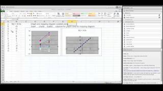
The sliders adjust the height of the second complex plane, the power, n, and the radius of the circle for the mapping diagram arrow source.


Thanks¤.

Questions?

The End!


http://flashman.neocities.org/Presentations/MD.Reed.CV.9_19_16.html


References:¤

Mapping Diagrams from A(lgebra) B(asics) to C(alculus) and D(ifferential) E(quation)s.
A Reference and Resource Book on Function Visualizations Using Mapping Diagrams

The Sensible Calculus Program