Chapter IX: DIFFERENTIAL EQUATIONS AND POLYNOMIALS: TAYLOR'S
THEOREM
© 2000 M. Flashman
In numerous cases throughout this book, as in the
real world, we find problems
where an exact numerical answer is either impossible or impractical to
express as a decimal number. Examples of these situations include
calculation
of `sqrt{2}, pi, e` , and `ln(2)`. As we have seen there are many ways
to characterize and
define
these numbers and use these characterizations to find an estimate. For
our discussion in this chapter it is important to notice that each of
these
numbers can be characterized as arising from the evaluation of a
function
which is the solution to a differential equation.Euler's method is one
way we have studied to make these estimates. [See Table 1 below.]
|
NUMBER
|
FUNCTION
|
DIFFERENTIAL
EQUATION
|
|
$\sqrt{2}= f(2)$
|
$f(x) = \sqrt{x}$
|
`f ' (x) = 1/ {2f (x)}, f (1) = 1`
|
|
`ln(2) = f(2)`
|
`f(x) = ln(x)`
|
`f ' (x) = 1/ x, f (1) = 0`
|
|
`e = f(1)`
|
`f(x) = e^x`
|
`f ' (x) = f (x), f (0) = 1`
|
|
`pi =
f(1)`
|
`f(x) = ` 4arctan` (x)`
|
`f ' (x) = 4/{1 + x^2}, f (0) = 0`
|
We have discussed approximations from the very beginning of our
work on
the derivative, with Newton's method for estimating the roots of
equations,
Euler's method for estimating particular solutions to differential
equations,
and numerous methods for estimating definite integrals. In the
following
sections we will delve further into the nature and applications of
polynomial approximations
based on information about the derivatives of a function.
We shall refer to these polynomial approximations as Taylor's
approximation theory. To provide further motivation let's consider
first a simple situation where
an exact value for a function is attainable but perhaps not worth the
effort.
EXAMPLE IX.A.1: Suppose `f (x) =x^2 + x^3 + x^100`
and
we wish to find
`f (0.5)`.
Of course the exact answer is `.25 + .125 + (.5)^100`, but if
we only need an estimate of the answer it is easy to settle for .375.
The
error we make in using this estimate is relatively small [namely
`(.5)^100`].
In this example we should note two things.
- First, the computation for the estimate is theoretically easy
because the function involved
is a polynomial; and
- second, the estimate was found by evaluating a related
polynomial, `g(x) = x^2 + x^3` .
Taylor's Theory-Objective and Key Ideas: The main concerns
of Taylor's theory for estimating function values are
- to find estimating polynomials for a given function and
- to measure the error in using these polynomials to estimate the
desired
values
for
the given function.
Two Key Ideas: You may recall from our earlier discussions of
estimations
using the differential that when `x` is close to `a, f(x)` is
approximately
equal to a linear function, `f(a) + f '(a) (x-a)`. Furthermore,
the Mean Value Theorem guarantees that as long as `f `is a sufficiently
well behaved function there is some `c` between `a` and `x` where `f(x)
- f(a) = f '(c)(x-a)`. Thus the difference between the function's
value at `x` and `a` can be measured using the value of the derivative
of `f` at `a`..
Taylor's theory generalizes these two ideas that use the derivative
to estimate.
IX.A. Estimating `e^x` with Polynomials: An
Introduction
to Taylor's Theory.
To focus our discussion more specifially, in this section we will
consider
only `f(x)=e^x`and begin by trying to estimate `f(1)=e` illu
strating the key ideas
of
Taylor's theory.
At `x = 0`, we find that `f(0) =1`, `f '(0) =1`, and since
`f
'(x)
= f(x)` we have that `f^{(n)}(0) =1` for all
natural numbers `n`. We now consider our first result, typical of
the Taylor's theory approach to estimation using polynomials and
derivative
information.
PROPOSITION IX.A.1: If `P_n(x)= 1 + x+ {x^2}/2 +
{x^3}/{2*3} + {x^4}/{4!}+...+{x^n}/{n!}`
then
`P_n(x)` is a polynomial of degree n
so that `P_n(0)= P_n'(0)=P_n''(0)=...=P_n^{(n)}(0)=1`
and `P_n(b)` is approximately equal to `e^b`.
In
fact, if we let `R_n = e^b - P_n(b)`, then for some `c` between
`0` and `b`, `R_n = e^c {b^{n+1}}/{(n+1)!}`
.
GeoGebra: Table, Graph, and Mapping Diagram of `P_n(x)` and `R_n(x)`
Estimating e: Before we proceed to justify this result,
we'll
apply
this result using `n=5` to estimate the value of `e [=e^1]`.
First, `P_5(x)= 1 + x+ {x^2}/2 + {x^3}/{2*3} +
{x^4}/{4!}+{x^5}/{5!} = 1 + x+ {x^2}/2 + {x^3}/{6} +
{x^4}/{24}+{x^5}/{120}` ,
so according to the proposition, `e` is approximately equal to
`P_5(1)=1 + 1+ {1^2}/2 + {1^3}/{6} + {1^4}/{24}+{1^5}/{120} ~~
2.716667` and
`R_5 = e-P_5(1)` where `R_5 = e^c {1^6}/{6!}=e^c 1/720` for some `c`
between `0` and `1`. Thus, `e` is approximately `2.716667` and the
error
in using this estimate is `R_5`. Since `c` is between `0` and `1`,
`e^c`
is between `1` and `e`, so we can deduce that `R_5`, the difference
between e and the estimate, `P_5(1)`, is no greater than `e/720`. Using
estimates of `e` from our earlier work in Chapter VI we know
that `e< 3` so our error `R_5(1)` is no larger than `3/720 = 1/240
\approx 0.004167`.This compares roughly well with the error from the
GeoGebra applet that shows an error after setting the slider $n = 5$
to find `R_5(1) = 0.00162`.
A more accurate estimate can be obtained by using a larger value
for
`n`. Try using `n=6` and `7` to see the improvement. [This can be done
progressively
using the GeoGebra applet above or download a spreadsheet
which
you can examine now or later.]
Proof of Proposition: We'll begin our proof by finding
`P_n'(x)`.
`P_n'(x)=1+ x+{x^2}/2 +{x^3}/{2*3}+{x^4}/{4!}+...+{nx^{n-1}}/{n!}`
`= 1 + x+ {x^2}/2 + {x^3}/{2*3} +
{x^4}/{4!}+...+{x^{n-1}}/{(n-1)!}=P_{n-1}(x)`
From this it follows easily that `P_n(0)=
P_n'(0)=P_n''(0)=...=P_n^{(n)}(0)=1`.
Now suppose that `b` is not `0` and let `R_n = e^b
-
P_n(b)`.
We need only justify the formula for evaluating `R_n`.
For convenience we'll write `R=R_n` and let
`g(t) = e^t P_n(b-t) + R{(b-t)^{n+1}}/{b^{n+1}}`.
Then `g(b) = e^b P_n(b-b) + R{(b-b)^{n+1}}/{b^{n+1}}= e^b P_n(0) = e^b`
,
while
`g(0) = e^0 P_n(b-0) + R{(b-0)^{n+1}}/{b^{n+1}}=P_n(b) + R = e^b`
from the definition of R.
Furthermore `g'(t) = e^t P_n(b-t) - e^t
P_n'(b-t)-R{(n+1)(b-t)^{n}}/{b^{n+1}}=e^t[P_n(b-t) -
P_n'(b-t)]-R{(n+1)(b-t)^{n}}/{b^{n+1}}`
But `P_n(x) - P_n'(x) = {x^n}/{n!}`, so`g'(t) = e^t
{(b-t)^n}/{n!}-R{(n+1)(b-t)^{n}}/{b^{n+1}}`.
Now we apply the Mean Value (or Rolle's) Theorem to the function g,
we
can
say
that there is a number `c` between `0` and `b` where
`g'(c)=0`.
Thus
`0 = e^c {(b-c)^n}/{n!}-R{(n+1)(b-c)^{n}}/{b^{n+1}}`and `e^c
{(b-c)^n}/{n!}= R{(n+1)(b-c)^{n}}/{b^{n+1}}`.
Solving this last equation for R gives
`R_n = R = e^c {b^{n+1}}/{(n+1)!}`.
EOP.
Note: Since the exponential function has a positive
derivative for all `x`, the function is increasing for all
`x`.
(i) If `0<c<b` then `1< e^c < e^b < 3^b` and `0 <
{b^{n+1}}/{(n+1)!} < R_n = R = e^c {b^{n+1}}/{(n+1)!} < e^b
{b^{n+1}}/{(n+1)!}< 3^b{b^{n+1}}/{(n+1)!}`.
(iia) If `0>c>b` then `1> e^c >e^b > 2^b` and if `n`
is odd then `{b^{n+1}}/{(n+1)!` is positive and thus
`{b^{n+1}}/{(n+1)!} > R_n = R = e^c
{b^{n+1}}/{(n+1)!} > 2^b {b^{n+1}}/{(n+1)!} > 0`.
(iib) If `0>c>b` then `1> e^c >e^b > 2^b` and if `n`
is even then `{b^{n+1}}/{(n+1)!` is negative and thus
`{b^{n+1}}/{(n+1)!} < R_n = R = e^c
{b^{n+1}}/{(n+1)!} < 2^b {b^{n+1}}/{(n+1)!} < 0`.
Putting this information about the quality of `R_n` together we can see
the following:
For all `x > 0` and for any `n`, `e^x > P_n(x)`,
while for ` x< 0` the polynomials differ in relation to `e^x`:
When `n` is odd then `e^x > P_n(x)`;
when `n` is even then `P_n(x) > e^x`.
Estimating the
value of e is not the only use for the previous proposition.
Before turning to the more general Taylor's theory in the next section,
here are two more examples of its application in estimating definite
integrals
related to ex.
EXAMPLE IX.A.2: Estimate `int_0^1 e^x dx = e-1`.
Use this to estimate `e`.
Solution: Using Proposition IX.1 with `n=4` for each x
between `0` and `1` we have
`0<e^x =P_4(x) + R_4(x) = 1 + x+ {x^2}/2 + {x^3}/6 +
{x^4}/24+R_4(x)` where `R_4(x) = e^c {x^5}/120`
for some `c` with `0<c<x<1`.
Thus`0<R_4(x)<3 {x^5}/120 = {x^5}/40`.
[Remember `e^c<3`.] and so `P_4(x)<e^x<P_4(x) + {x^5}/40`
for all `x` between `0` and `1`. Now we use the monotone property of
the
definite integral [Ch. V . ** ] to obtain the estimate:
`int
_0^1P_4(x)dx<int_0^1e^x dx<int_0^1P_4(x) + {x^5}/40`,
so
`1+1/2 + 1/6+1/24+1/120< e-1<1+1/2+1/6+1/120+1/240`.
Therefore `e` is approximately `1 + 1+ 1/2+1/6+1/24+1/120
~~2.716667`
as in the first estimate we saw in the note after the statement of the
theorem, and the error in using this estimate is less than `1/240`
as we also saw previously.
The next
example follows a similar analysis but applied to a more
difficult
yet important integral for probability and statistics.
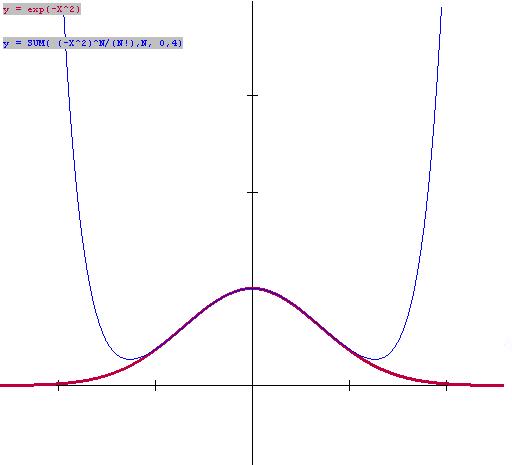
EXAMPLE IX.A.3: Estimate `int_0^1 e^{-t^2}dt`.
Solution: For each `t` between `0` and `1`, `-t^2` is
between `-1` and `0`. Let `x = -t^2`. By Proposition
IX.1 with `n = 4` for each `x` between ` -1` and `0` we have
`0<e^x =P_4(x) + R_4(x) = 1 +
x+
{x^2}/2 + {x^3}/6 +{x^4}/24+R_4(x)`
where `R_4(x) = e^c {x^5}/120` for
some
`c` with `0>c>x`.
Since `c<0` , `0<e^ c<1`, and since `x < 0` we
have that `0>R_4(x)>{x^5}/120`.
|
|
| GeoGebra Estimates for `int_0^1 e^{-t^2}dt`. Check off box to show estimate.
|
|
Substituting `-t^2` for `x` ,we see that
`e^{-t^2} = 1 + (-t^2)+ {(-t^2)^2}/2 + {(-t^2)^3}/6
+{(-t^2)^4}/24+R_4(-t^2) = 1-t^2+{t^4}/2 -{t^6}/6 +{t^8}/24 +
R_4(-t^2)`
Now since `0>R_4(-t^2)>{(-t^2)^5}/120 ={-t^10}/120` we have
`int_0^1 P_4(-t^2)dt >int_0^1 e^{-t^2} dt > int_0^1 P_4(-t^2)
-{t^10}/120 dt`.
By evaluating these integrals we obtain
` int_0^1 1-t^2+{t^4}/2 -{t^6}/6 +{t^8}/24 dt > int_0^1e^{-t^2}dt
> int_0^1 1-t^2+{t^4}/2 -{t^6}/6 +{t^8}/24 - {t^10}/120 dt`
or `1- 1/3 + 1/10- 1/42+ 1/216 > int_0^1e^{-t^2}dt > 1 - 1/3
+ 1/10- 1/42+ 1/216 - 1/1320`
Therefore, `int_0^1 e^{-t^2}dt`
is approximately equal to `1 - 1/3 + 1/10 - 1/42 + 1/216 ~~
0.747486...`;
and this is an overestimate by no more than `1/1320`.
Comment: In both of these examples we have been able to
estimate
a definite integral involving the exponential function by using a
Taylor
polynomial of degree 4. It should be apparent that by using a higher
degree
for the estimating polynomial, the error term will become smaller and
we
will obtain a more precise estimate. The systematic pattern in these
polynomials
should allow you to find more precise estimates for the last example
without
much difficulty.
Go on to Chapter IX.B
Exercises IX.A.:
- Use the Taylor polyonmial for `e^x` of degree `4` to estimate
the
following:
(a) `e^2` (b) `e^3` (c) `e^.5` (d) `e^-1` (e) `e^3.14`. [Use GeoGebra or Spreadsheet
helper.]
- Estimate e using the Taylor polynomial of degree n where
n is (a)
6 (b)
7 (c) 8 (d) 10.
In each of these estimates discuss the size of the error term Rn.
[Use GeoGebra or
Spreadsheet
helper.]
- What value of n should be used so that the Taylor
polynomial of
degree
n will give an estimate of e that is within .000001 of the exact value
of e? Explain your result using Proposition XI.A.1
- Use the Taylor polynomial for ex of degree 5 to
estimate
`int_0^1 e^{-t^2}dt`.
Discuss the error in this approximation.
- Use the trapezoidal rule and Simpson's rule with n = 6 to
estimate `int_0^1 e^{-t^2}dt`
.
- Use the Taylor polynomial for `e^x` of degree 6 to estimate
`int_0^1 e^{-t^2}dt`. Discuss the error in this approximation.
- On the same graph sketch the graph of `e^x` along with those for
the Taylor polynomials for `e^x` of degree
1,2,3,4 and 5. [You can do this by use the trace feature on the graph of
`P_n` in the GeoGebra applet.] Discuss the graphical interpretation
of `R_n`. [Here is Java
sketch
solution
for
n = 1 to 5]
- What value of n should be used so that the Taylor polynomial of
degree
n will give an estimate of `int_0^1 e^{-t^2}dt` that
is within `0.000001` of the exact value? Explain your result.
- Use the Taylor polynomial for `e^x` of degree 4 to estimate the
area of the region in the plane contained by the lines `X=0`, `X=1`,
the X-
axis and the graph of `y = 1 + xe^{-x}` . [Hint:
First find a polynomial to estimate `e^{-x}` .] Discuss the
error in this approximation.
- Another Polynomial Estimate: Consider the functions `1/{1-x}`
and
`1/{1+x}`.
- Show that `1 = (1-x ) ( 1 + x + x^2+ x^3+x^4+ x^5) + R` where
`R =x^ 6` .
- Show that `1 = (1+x) ( 1-x + x^2 - x^ 3+x^ 4 - x^ 5) + R`
where `R = x^ 6` .
- Show that when `0 < x< 1, 1/ (1- x) = ( 1 + x+ x^ 2+ x^
3+ x^ 4+ x^ 5 ) + R_1` where `R_1 = {x^ 6} /{ 1-x}`
- Show that when `0< x < 1, 1/ {1+ x} = ( 1 -x+ x^ 2 - x^
3+ x^ 4 -
x^ 5 ) + R_2 ` where `R_2 = {x^ 6}/{1+ x}`.
- Use the definite integral and the previous equations to
estimate ln(.9)
= ln (1 - .1) and ln(1.1) = ln(1 + .1). [ This approach to estimating
the
natural logarithm was used
by Isaac Newton to give very accurate estimates of ln(2), ln(3),
etc.].
Discuss the error in your estimate based on the integrals of R1
and R2.
- Generalize this for higher degree polynomials and estimating
ln(.8),
ln(1.2),
ln(.99) and ln(1.01).