August 2008:
This page now requires Internet Explorer 6+
MathPlayer
or Mozilla/Firefox/Netscape 7+.
CHAPTER IV
Differential Equations from an Elementary Viewpoint
© 2000 M.
Flashman
Preface: Some thought experiments. We
begin this chapter with some model contexts.
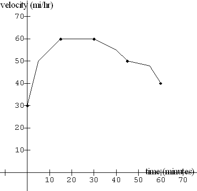
| [Motion based model] Think of driving a car along a road.
Your odometer
is broken but your speedometer still works. You record only where the
car
is when you begin your trip and you make a table of the car's speed
(velocity)
at regular time intervals during the trip. [Or perhaps you can record
the
velocity at every time from the beginning to the end of the trip].
Based
on this information do you think you could give your location
approximately
(or exactly) at any time during your travels? As a practical matter, if
you have the time to repeat the trip this shouldn't be too difficult.
With
the information you recorded you can reproduce the trip with some
accuracy.
This time use a car with an odometer and let someone else do the
driving
according to the recorded velocities while you record your
position.
For an hour trip this might be more time than you want to
spend on this.
With a little thought and few arithmetic calculations, you should
become
up with a reasonable estimate of where you were at the same points in
time
where you recorded the velocities.
|
Table of Velocities Read from Speedometer during
Trip
|
t minutes
|
v(t) miles/hour
|
|
0
|
30
|
|
15
|
60
|
|
30
|
60
|
|
45
|
50
|
|
60
|
40
|
Click here
to see a position function that matches these instananeous velocities. |

Graph of Velocities
Read from Speedometer during Trip
|
| [Motion based model] Next suppose you
are driving
on a highway through a major city. (Los Angeles, Chicago, New Orleans,
Miami, or New York will do). You are trying to explain to your
passenger
why you are travelling at your current speed. What would you include in
your explanation? The time of day (6 a.m. or 6 p.m.)? Or the position
in
the road ( before a major interchange, on a stretch where construction
is under way, or on a section where two additional lanes have been
added)?
Or perhaps the speed at which other vehicles are travelling ( you are
travelling
up a hill behind two large trucks)? Based on this information can you
tell
your passenger where you will be in the next few seconds, minutes,
hours?
How accurate will your predictions be? |
Table of Speeds on Highway 51 South through the City
of Ush
at various times of day.
time\ Mile marker
on highway
|
5
|
8
|
10
|
12
|
|
6:00
|
60
|
55
|
50
|
60
|
|
8:30
|
40
|
40
|
25
|
50
|
|
11:00
|
50
|
50
|
45
|
55
|
|
15:00
|
55
|
50
|
45
|
60
|
|
18:00
|
40
|
30
|
35
|
40
|
|
23:00
|
60
|
60
|
50
|
60
|
|
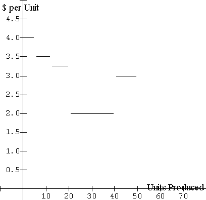
| [Production based model.] Think of manufacturing a very
desirable product,
"good stuff." As your production increased you forgot to keep track of
your accumulated costs but you did keep your receipts showing you the
marginal
rates you were charged for materials and labor. Based on this
information,
do you think you could give your accumulated costs approximately (or
exactly)
at any stage of the production? As a practical matter, this is what
accountants
do in reviewing the accumulation of costs. With the information you
have
retained you should be able to reproduce the accumulation of costs with
great accuracy. |
Units
produced
|
Marginal cost
$/ unit
|
|
0 to 5
|
4.00
|
|
5 to 12
|
3.50
|
|
12 to 20
|
3.25
|
|
20 to 40
|
2.00
|
|
40 to 50
|
3.00
|
Click here
to see an accumulated cost function that matches these marginal costs
|

Graph of Marginal Cost
per Unit Produced
|
[The Dart Model] Suppose you are throwing a dart at a region
in the
plane and measuring a random variable X determined by the position of
the
dart. X has values only between 0 and 10. Unfortunately you are not
given
the distribution function of X. [Recall that for any real number A
between
0 and 10 the distribution function F, would give you F(A), the
probability
that the value of X is less than or equal to A.]
Instead you have been given a graph, an algebraic expression and a
table for the probability density function of X. [Recall that for
any real number A between 0 and 10 the probability density
function
of X, f, gives you f(A), the derivative of F at
A,
which is approximately the ratio of the probability of the random
variable
X being in an interval [A, A+h] to the length of that interval, h.]
Based on this information do you think you could estimate the
probability
that the value of X being less 5? Recognizing that F(0) = 0 and F(10) =
1, could you estimate F(A) for any A between 0 and 10? As a practical
matter,
you might break the interval into10 pieces of equal length and then
estimate
the probability of X being in each of those interval from the density
of
X at some point in that interval. Then for A, just add up the
probability
estimates for X being in an interval that has values less than or equal
to A. |
| A |
f (A) |
| 0.5 |
.05 |
| 1.5 |
.13 |
| 2.5 |
.11 |
| 3.5 |
.15 |
| 4.5 |
.19 |
| 5.5 |
.17 |
| 6.5 |
.09 |
| 7.5 |
.07 |
| 8.5 |
.03 |
| 9.5 |
.01 |
Click here
to see a probability distribution function for X that matches these
probability
densities. |

Graph of data for f(A)
The Probability Density Function for X
|
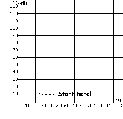
| [The Treasure Hunt] Here's another context. You are on a
treasure hunt.
Besides telling you where to start and which way to go, the directions
tell you the speed and direction you should travel and how long you
should
follow that instruction. Could you find the treasure? Would you be able
to tell where you were at any time during this trip? |
The
Treasure Hunt Directions
Start at
(20,10) on the
map.
- Head
north at 3 feet per second
for exactly 20 seconds.
- Now
turn
east and proceed at
2 feet per second for 10 seconds.
- At
this
point head south at
4 feet per second for 5 seconds.
- Turn
and
proceed due west at
one foot per second for 8 seconds.
You
should be at the
treasure now! Good luck.
|
|

Click on this map
to find the treasure.
|
Though these illustrations may
seem
a little artificial, the contexts reflect many real circumstances.
Often
we know something about the rate at which some measured quantity (e.g.,
rain, snow, population of owls or fruit flies, people infected with a
virus,
chemical, or money) is changing. Using these rates (i) we would
like to know the quantity present at certain times, i.e., when
t
= a, find f (a); or (ii) we would
like
to predict when the quantity will reach certain levels (either
desirable
or undesirable), i.e., given c, find b
so that when t = b, f(b) = c.
Here
are
two key questions:
- How does the rate of change for quantities control the
actual
amounts of
those quantities as they change? and
- What controls the rates of change?
Scientific investigators and engineers look for relations that
determine
rates of change in real contexts along with specific measurements from
which the information can be extended, by interpolation or
extrapolation.
The mathematical investigation of rates using calculus is the
defining
objective for the study of differential equations. This is one of
the
most important and, therefore, most studied parts of mathematics. It
will
be a major theme for the remainder of this book. You should note that
this
is not our first discussion of rates and related contexts. In our study
of implicit differentiation and problems with related rates we
encountered
many equations involving derivatives of varying complexity. Often the
derivative
in these studies depended on both the x and y
variables.
For example, implicitly differentiating the equation y3
=
x2
with respect to x leads to the derivative equation, dy/dx
= 2x/3y2. Differentiating the same
equation
with respect to the variable t (which is not expressed in the
equation)
leads to the derivative equation 3y2 dy/dt
= 2x dx/dt. [In fact, we could also express
these
last two situations with one equation using differentials: 3y2
dy = 2x dx.]
In this chapter we begin our examination of
differential
equations and some of the basic solution concepts for these equations.
In doing this we will use our previous work on the derivative (and
differentials)
to explore these concepts visually, numerically, and symbolically. Our
purpose
is
to develop some systematic methods (a calculus) for solving
differential equations. As we proceed through the chapter we will
follow
a recurrent path of
- examining cases that are simple and known with a new tool
for
understanding
a differential equation,
- describing how the tool is managed with some generality, and
- applying the tool to cases where previous techniques are not
as
successful.
IV. A. Differential Equations. Basic Concepts
and Definitions.
A differential equation (D.E.) is
an
equation involving derivatives in its statement. Here are some
examples:
| (i) dy/dx = x 2 |
(ii) y' - x + x 2 = 3xy |
| (iii) y' + xy = (y') 2 |
(iv) f ''(x) = 5 |
| (v) p''(x) +xp'(x) + p(x) =
0 |
(vi) Dt f(t) + t f(t)
=
3 |
| (vii) y'' + y' = 5 + y''' |
(viii) du/dt + dv/dt = 5 |
A differential equation involving only first derivatives is called a
first
order differential equation. Examples (i)-(iii), (vi), and
(viii)
are all first order differential equations. When no higher than
the second derivative is involved in the equation it is called a second
order differential equation. Examples (iv) and (v) are
second
order differential equations. Higher order differential equations
involve
higher order derivatives. As you might guess at this point, equation
(vii)
is a third order differential equation.
In some situations a differential equation may be expressed using
differentials!
For example, the equation dy/dx = x2/y
might be expressed as dy = x2/y dx
or as y dy = x2 dx.
Interpretation: We have seen that
a derivative can be interpreted dynamically as a rate of change (of
various
orders) or geometrically as the slope of a tangent line. Following the
dynamic view, a differential equation can be interpreted as a relation
between measured quantities and their rates of change. Understanding
these
relations is at the heart of most questions in the sciences. A
scientist
studies not only what things are but also how things change. An
understanding
of change allows scientists (and engineers) to predict and thereby
control
different aspects of our world. This is easy to believe in the
physical,
chemical, and biological science, but it is increasingly true as well
in
such disciplines as economics, management, geography, and other social
sciences. You can find contexts for using differential equations almost
anywhere you look.
Differential equations for motion were among the early
motivations for
developing the calculus. Today the need to analyze and control change
in
complex situations is a major reason why the study of calculus and
differential
equations is considered so important. These equations are used to study
everything:
- from the forces in the smallest subatomic particles, to the
motion of space
craft,
- from the growth of small cell and insect populations to the
complex interrelations
of environmental systems,
- from the effect of a sudden cooling on a hot summer day to
the
global effects
of a hole in the ozone layer of the atmosphere, and
- from the profitability of a single business decision to the
effect of major
fiscal and monetary policy changes on national and international
economics.
Be it mechanics, heat, sound, light, or the price of butter in
Burbank,
whatever the subject, there is usually one or more differential
equations
useful in its study. It is should be no surprise then that so many
disciplines
require their students learn calculus.
| I am sure you know what it means to solve an equation in
algebra. It
means to find all those values chosen from a given set of possible
solutions
that will make the given equation true. So, for example, 2 and -2 are
the
solutions from the set of integers for the equation x2 = 4.
Similarly, the equation sin(t) = 0 has an infinite set of solutions
when
we allowing real numbers as possible solutions, namely {`t = 2 pi k`
where k is any integer}, but this same equation has only one solution
that
is a rational number, namely 0. |
A solution to a differential
equation
with one dependent variable is a differentiable (hence, continuous)
function
which satisfies the differential equation on an interval domain.
Thus y = x 3 / 3 + 5 is a solution
to the differential equation dy/dx = x 2.
This
solution
is not unique, since y = x
3/3 - 9 will satisfy the same differential equation.
As a second example you can check that `y = sqrt{25 - x^2}`
on
the interval (-5,5) and `y = sqrt{16 - x^2}`on
the interval (-4,4) are both solutions to the equation dy/dx
= -x/y. With these examples we can identify two key
issues
in the study of differential equations.
Issue I:
When
does a differential equation have a solution?
Issue II: How unique is the solution of a
given differential equation?
We observe as a first response to these issues that it is easier to
check
whether or not a function is a solution to a given differential
equation
than it is to find a solution.
The general solution to a differential equation is
the
family of all functions that are solutions to a given differential
equation.
For example, the general solution to the differential equation dy/dx
= x 2 is the family of functions of the form y
= x3 / 3 + C where C is a constant.
[This
statement should seem plausible at this stage. It will be justified in
Section
IV.B.1.] The general solution to the equation dy/dx
= -x/y is the family of functions of the form `y =
+-sqrt{a^2 - x^2}` on
the interval (-a, a) where a>0 is a constant.
[This
statement will be justified in Chapter VII.]
We can now identify a third key issue in the study of
differential equations,
one that focuses not on existence or uniqueness of a solution, but on
the
ability to describe a solution in familiar terms.
Issue III: Is it
possible to describe the general solution to a differential equation as
some elementary function?
This is not always possible. For example, there is no description
possible
for the differential equation dy/dx = sin(x2)
as an elementary function.[This result is not easy to justify.] For
that
reason we are also interested in describing the general solution
graphically
and estimating values for solutions numerically.
Conventions in Language and Notation:
When the differential equation has the
form y' = P(x) where P is a function of x only,
the general solution is also called the indefinite integral of
P(x) or the anti-derivative of P(x) and is
denoted
`int P(x) dx`.
[N.B. In this situation the variable y does not
control
the derivative, y'.]
This is usually read as "the (indefinite) integral of P(x)
with
respect to x " or more simply "the (indefinite) integral of P."
[The word "indefinite" is frequently omitted.]
P(x) is called the "integrand" of the indefinite
integral.
[The significance and utility of this notation will become more
apparent
later.] The process of finding the general solution in this case is
called
"integration."
Continuing the previous example, writing `int
x^2
dx = 1/3 x^3 + C` is understood to mean that the indefinite
integral of the
function given by the rule x 2 with respect to
variable
x
is the family of functions of the form `1/3
x^3 + C` where `C` is a constant.
[This follows the conventional
abuse of notation: name a function by its rule and then announce the
controlling
variable for the rule.] In the general solution, the term "`C`"
is
described
as a constant of integration.
It might be more correct to write `int x^2 dx =`
{`1/3 x^3 + C` : where C is any constant
}.
The braces here indicate that we are describing a
family
of functions as opposed to one generic member of the family. This
notation
is not conventional and we will continue in the text to ignore this
overly
refined view. Remember that in conventional notation there is some
ambiguity
in representing the family of functions by a single generic member.
As the remarks in the preface to this chapter
indicated, knowing where you start on a trip determines in part where
you
will be subsequently. Often a differential equation has one or more
additional
conditions which a solution must satisfy as well, such as y(0)
=
7 or y(3) = 4. Additional conditions often arise in
applications
from information given about the beginning of a situation ("initial
conditions")
or conditions that must be satisfied at the beginning and end of the
process
("boundary conditions"). Such conditions restrict the selection of
solutions
to only a few particular members from the family of all solutions. A particular
(or special) solution to a differential equation is a
solution
that satisfies any such additional conditions.
Continuing with our example of the differential equation dy/dx
= x 2, we suppose that the general solution is y
= x 3/3 + C. If we use the initial condition y(0)=7
with
this
situation, it must be that
7 = (0) 3/3 + C, so C = 7.
Thus the particular solution to this differential equation with the
given
initial condition is y = x 3/3 + 7. [This is
easily
checked by finding the derivative, dy/dx, and evaluating
y
when x = 0.]
Looking at the differential equation dy/dx = -x/y,
we
suppose
that the general solution is `y = +-sqrt{a^2 - x^2}`
where
a is a constant. If we use the condition y(3)=4 with this
situation,
it must be that `4 = y(3) = +sqrt{a^2 - 3^2}` ,
so `16 = a^2 - 9` and `a^2 = 25` and
therefore
`y = +sqrt{25 - x^2}` is
the particular solution to this differential equation with the given
condition.
Notice that in each of these examples there is only one function
that
will satisfy both the differential equation and the given initial
condition,
i.e., the solution in these special situations is unique.
Key Words: Look the following words up in a dictionary. Compare
the dictionary definition(s) to the use of the word in this section.
| differential |
equation |
boundary |
| solution |
antiderivative |
particular |
| condition |
integral |
general |
| initial |
indefinite |
unique |
PROBLEMS IV.A
1. For each differential equation determine whether or not the
given
function is a solution.
| a. dy/dx = 3x 2 - 2x +
5; |
y = x 3 - x 2
+ 5x
- 8. |
| b. y' + 2y = x 2 + 3x
+ 5; |
y = x 2 + x + 4. |
| c. dy = 12x cos(x 2) dx; |
y = 6 sin (x 2) + 25 |
| d. y dx + x dy = 4x
3 dx;. |
y = x 3 |
| e. y''= 12x 2 - sin(x) +
2; |
y = x 4 + sin(x) + x
2 + 3x + 5 |
| f. P''(t) + P(t) = 0; |
P(t) = 5 sin(t) - 10 cos(t) |
| g. d2 z/du2 - 9z = 0; |
z = e3u |
| h. g'(t)= 2/t + 3e3t ; |
g(t) = 2 ln(t)+ e3t |
2.The following table shows the velocity of a car during a trip on a
rural
highway recorded at 30 second intervals. Based on this information
estimate
the answer to the following questions. Explain your reasoning briefly.
Problem 2.
|
time (min)
|
0 |
.5 |
1 |
1.5 |
2 |
2.5 |
3 |
3.5 |
4 |
4.5 |
5 |
5.5 |
6 |
|
velocity (mi/h)
|
0 |
30 |
25 |
30 |
10 |
-15 |
-25 |
-10 |
25 |
40 |
50 |
50 |
30 |
a. How far was the car from its starting point after 3 minutes and
after
six minutes?
b. How many miles did the odometer change after 3 minutes and after
six minutes?
c. When during the trip did the car pass a point on the highway 3 miles
from the starting point?
d. When did the car turn around and head back to the starting point?
e. The car turned around because the driver wanted to check on the
name on a mailbox they had passed. Approximately where was the mailbox
located?
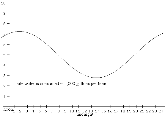
3. In the figure below is the graph of the rate at which water
was used
during a twenty four hour period in the town of USH. Based on the graph
draw a sketch of a graph showing the amount of water used as a function
of time during the same period. Estimate the amount of water consumed
during
the twenty four hour period.

4. Suppose that the general solution to the differential
equation
dy/dx
= 3x 2 + 5 is given by y
= x
3 + 5x + C where C is a constant. Determine the value
of C that will give a solution to this differential equation with the
given
condition.
(a) y(0) = 7 (b) y(0) = -4
(c) y(1) = 7 (d) y(1) = -4
5. Suppose that the general solution to the differential
equation
y''+
y
= 0 is given by y = Asin(x) + Bcos(x)
where
A and B are constants. Determine the values of A and B that will give a
solution to this differential equation with the given conditions.
(a) y(0) = 5 , y'(0) =
6 (b)
y(0)
= -3 , y'(0) = 4
(c) y(0) = 2 , y(p/2)=
3 (d) y(0) = -2 , y(p/2)=
5
In problems 6 and 7, do not try to solve the differential
equations.
Without knowing explicitly what y is as a function of x,
but
using
knowledge of its derivative from the differential equation, there
is still much you can say about y in these problems..
6. Assume y is a solution to the differential equation dy/dx=
x/(x
2 + 1) with y(0)=2.
(a) Using just the given information, find any local extreme points
for y and discuss the graph of y,
including
the issue of concavity.
(b) Using the differential, estimate y(1) and y(-1).
(c) Change the initial condition to y(0) = 3 and then y(0)=
1.
How
will these different conditions affect the graph of y? How
do they affect the estimates for y(1) and y(2) made in
part
b?
7. Assume y is a solution to the differential equation dy/dx=
y
- 1 with y(0)=2 and y(x) >1 for all x.
(a) Using just the given information, discuss the graph of y
including the issue of concavity.
(b) Using the differential, estimate y(1/2) and y(-1/2).
(c) Suppose that y(x) <1 for all x and y(0)
=
0.
How will these different conditions affect the graph of y?
How do they affect the estimates for y(1/2) and y(-1/2)
in
part b?
8. Match each indefinite integral with the family of functions
that
best describes it.
| (a) ∫ x3
dx |
(i) -x2/6+C |
| (b) ∫
3x dx |
(ii) (3/4)x4/3+C |
| (c) ∫ x-3
dx |
(iii) (1/4)x4 +C |
| (d) ∫ x1/3
dx |
(iv) (3/2)x2+C |
| (e) ∫
-x/3 dx |
(v) -x-2/2+C |
|
(vi) 3x4/3+C |
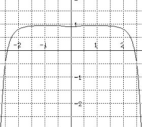
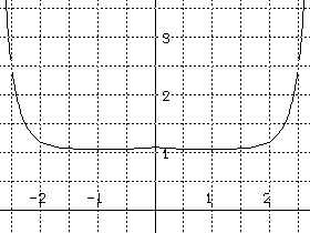
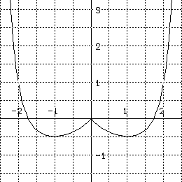
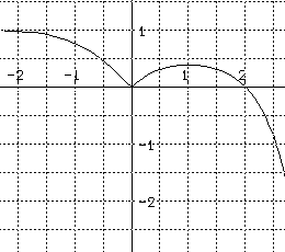
9. Assume y is a solution to the differential equation dy/dx=
(y-1)(x 2 -1).
(a) Assume that y(0)=2. Using the differential, estimate y(1/2)
and
y(-1/2).
(b) Change the initial condition on y to y(0) = 3 and
then y(0)= 1. How will these different conditions affect your
estimates?
(c) Which of the following graphs are likely to be the graph of a
solution
for this differential equation .


10. Match the following statements with the differential equation
that
best represents the situation described.
(a) As the runner approached the end of the race, she slowed her
rate
steadily so that when she crossed the finish line at 20 seconds she was
travelling at 7 meters per second.
(i) dr/dt = -7t+ 20 (ii) r'(t)=-kt + 7(t-20)
(iii)
dr/dt = -k(t-20) + 7
(b) The population of cells had a biomass of 30 milligrams when
the
experiment began. The biomass grew a rate proportional to the mass
present.
(i) P'(t) = k t (ii) P'(t) = k P(t)
(iii)P'(t)=
k (30 + P(t))
(c) The temperature of the coffee was initially 373 degrees
Kelvin while
the room was only about 333 degrees.. The coffee's temperature
decreased
at a rate proportional to the difference between its temperature and
that
of the room.
(i) dT/dt = -k (T-333) (ii) dT/dt = -k ( 373t
- 333) (iii) dT/dt = -k/(t-333)
(d) After 10 minutes the student was learning the material more
slowly
as time went on, so that his rate of learning was then decreasing
inversely
with the square of the time he had spent reviewing.
(i) dL/dt = k (t +10)2 (ii) DL(t) =
k/t2 (iii) L'(t) = k/(t+10)2
(e) The profits from the investment were increasing more slowly
as time
went on so that the rate appeared to decrease inversely proportionately
with the profits at any given time.
(i) P'(t)=k - P(t) (ii) DP(t) = k/t (iii)
dP/dt = k/P
(f) The marginal revenues from the production of more than 100
faucets
decrease proportionately with the number of additional faucets
produced.
(i) dR/dx = -kx (ii) DR(x) = -k(x+100)
(iii) R' = -k(x-100)
11. Which of the following equations mean the same thing? Explain
your
response.
∫4t3
dt
= t 4 + C; ∫4x3
dx
= x 4 + C;
D( t4 + C) = 4t3;
D(x4 + C) = 4x3
12. Use the interpretation of the derivative as the velocity of a
moving
object to explain the following statement: If two functions have the
same
derivative at every point then the difference between the values of the
functions at every point will be the same number.
13. Describe three contexts where the rate at which something is
used
is monitored to predict how much will be used in the future. Discuss
how
do these predictions affect planning?
14. The following table gives the speed of cars on a rural
highway at
the given time of day and the mile maker.
Problem 14. Table of Car Speeds.
\ time
mile marker |
5 a.m. |
8 a.m. |
11 a.m. |
| 10 mi. |
55 mph |
40 mph |
50 mph |
| 20 mi. |
30 mph |
20 mph |
30 mph |
| 30 mi. |
40 mph |
25 mph |
30 mph |
Based on this table estimate the time it takes to travel from mile
10 to
mile 40 at 5 a.m., at 8 a.m., and at 11 a.m. Discuss briefly the
assumptions
you made in making your estimates.
15. Sometimes it is possible to show that a differential equation
cannot
be solved by functions of designated type. For each of the following
differential
equations do not try to find a solution. Based on the equation
explain
why there can not be any polynomial function that would satisfy the
equation.
a) f '(x) = 5 f(x) and f(0)
=
2.
[Hint: Find a formula for f (n)(x). Show
that
f
(n)
(0)
is not 0 for any nth order derivative of f.]
b) f ''(x) = -5 f(x) and f(0) =
2.
c) dy/dx = 1/(1 + x2) and y(0)
= 2.
16. Suppose X is a random variable with range [0,10]. Give a
differential
equation that shows the relation of the probability density function f
(x)
and the distribution function F(x) for X. Explain briefly why
the
boundary conditions for this differential equation are F(0) = 0 and
F(10)=1.
Generalize this situation to a random variable with range [A,B].
