Section I.C. OTHER ESTIMATING CONTEXTS (draft)
© 2003, 2014 M. Flashman
Throughout the remainder of this book estimating a value of some quantity
will be a recurrent theme as it has been throughout the history of mathematics.
In Sections I.C.1 and I.C.2 we'll examine two more subject areas of both
historical and current importance that were introduced in Section
0.C, probability and economics. In these subjects estimations of the
type investigated with tangent lines and instantaneous velocity are also
relevant.If you are anxious to reach the mathematical concepts that these
models (along with those of Sections I.A and I.B) motivate you may proceed
now directly to section I.D. However, be sure to cover this section
before proceeding to Chapter II, as these models will serve as interpretations
for some of the later results in the text.
I.C.1 Probability Distributions and Density. In Section
0.C (which you might want to review now), we introduced some basic
concepts of probability with the darts model. To explore these ideas
further we'll continue our examination of that model. Recall that we were
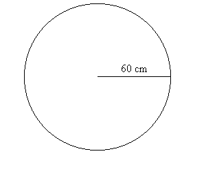
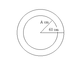
considering a circular magnetic board of radius sixty centimeters.
This magnet is very strong and uniformly attracting so that when I
turn my back to it and release a magnetic dart, the dart will be drawn
to the board and is equally likely to land on any point on the board.
This is our basic experiment. After performing the experiment we
measured the random variable $R$, the distance from the dart to the center
of the circle.
|  |
Notation: As in Chapter 0.C we will denote the probability
that the random variable $R$ has a value less than or equal to $A$ by F($A$)
where $A$ is any real number.
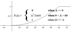
F is a function of $A$ called the (cumulative) probability distribution
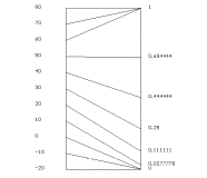
function for the random variable $R$. When analyzed by cases we saw that
$ F($A$) =
\begin{align}
0 \ \ \ \ \ \ \ \ \ \ \ \ \ \ \ \ A\le0 \\
\frac {A^2}{3600}\ \ \ \ \ \ \ \ \ 0 \lt A \lt 60 \\
1 \ \ \ \ \ \ \ \ \ \ \ \ \ \ \ \ 60 \le A \end{align}$
.
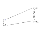
See Figures *** and *** for a mapping diagram and graph of this function. |
 |
 . . |
 |
We also saw in Section 0.C that the probability of the random variable
$R$ being precisely any specified value is always $0$. A related and
important issue is how to measure the likelihood of the dart landing
close to or equal to a particular distance, $A$, from the center of the
dart board. To be more specific, how can we measure the likelihood that
the value of $R$ would be close to or equal to $A=50$ centimeters? And
can we compare this to the likelihood that the value of $R$ would be close
to or equal to $A=10$ centimeters? The actual probability of these events
depends on the value of $A$ and the length of the interval that is
considered "close" to $A$.
Example
I.C.1.For our discussion, let's consider the dart falling close to
50 centimeters from the center as meaning that $R$ is in the interval [49,51],
and falling close to 10 centimeters as having $R$ in the interval [9,11].
The probabilities for $R$ being in these intervals is computed as in Section
0.C:
F(51) - F(49) = 512 / 3600 - 492 /3600
= 200 / 3600 = 1/18 for the interval [49,51],
and F(11) - F(9) = 112 / 3600 - 92 / 3600
= 40 / 3600 = 1/90 for the interval [9,11].
These measurements do not resolve the dart issue very well since the probabilities
change with the choice of the intervals used to determine what "close"
means. (What if we had used the interval [49.9,50.1]? ) To resolve the
issue of relative likelihood of the dart falling a certain distance from
the center, we will develop the concept of point probability density.
Point Probability Density: Recall from Section 0.C that the
average probability density (APD) of a random variable $R$ for
an interval [A,B] is the ratio of the probability that A< $R$ < B to the length of the interval $[A,B]$, i.e.,
$APD(A<B)=\frac {F(B)-F(A)}{B-A}$
|
 |
So the APD of $R$ in the interval $[29,31], APD(29,31) = (1/18)/2 =
\frac1 {36}$ and for the interval $[9,11]$ the $APD(9,11)= (1/90)/2 = \frac 1{180}$
Definition: The (point) probability density (PD) of a random
variable $R$ for a value $A$, denoted $f (A)$, measures the likelihood
that $R$ will take a value close to $A$. This number is estimated by
average probability densities for very short intervals with $A$ as one endpoint.
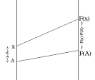
Let $\overline f(x)=\frac {F(x)-F(A)}{x-A} = APD(x,A)$, the APD for $R$ on an interval with endpoints $A$ and $x$ where $x$ is different from $A$. The preceding statements
can be expressed by saying that as $x$ approaches $A$, the values of $\overline f(x)$
should approach $f (A)$, i.e., as $x \rightarrow A$, we should find
that $\overline f(x) \rightarrow f(A)$. |
|
Note:
This method is very similar to the way that average velocities for very
short time intervals estimate the instantaneous velocity of a moving object,
or that the slope of a secant line for a short interval estimates the slope
of the tangent line to a curve.
We'll
continue the example that illustrates the meaning of this by determining
the point probability density of $R$ for the values $A=50$ cm. and $A
= 10$ cm. [You might pause a minute here and make your own estimates for
these numbers.]
EXAMPLE I.C.1. (Cont'd.) In the darts experiment described above
and in Example 0.C.3 with the random variable $R$, we find the average probability
density for $R$ for the intervals $[49,50]$ and $[50,51]$ to estimate the point
probability of $R$ at $50$ cm.
Using the probabilities from the previous discussion, we find the average
probability density for $[49,50]$, $APD(49,50)= 99/3600 = 11/400$, while
the $APD(50,51) = 101/3600$.
We continue to examine more closely the APD for intervals with 50 as
an endpoint in an attempt to determine whether some number can be assigned
as a point probability density to the number 50. Figure
I.17 shows a table of APD's for intervals with one endpoint being 50.
Figure I.17
Table of APD's for intervals with one endpoint being 50
| Interval |
Average Prob.Density |
| [49,50] |
99/3600 |
| [49.9,50] |
99.9/3600 |
| [49.99,50] |
99.99/3600 |
| [50,51] |
101/3600 |
| [50,50.1] |
100.1/3600 |
| [50,50.01] |
100.01/3600 |
Letting $\overline f(x)=$ the APD for $R$ on an interval with endpoints 50 and $x$ where $x$ is different
from 50, we have that
$\overline f(x)
= [ x^2/3600 - 2500/3600] / [x -50]$
$= [(x+50)(x-50)] /[3600 (x-50)]$
$= [x + 50]/ 3600$ .
Thus as $x \rightarrow 50, \overline f(x) \rightarrow \frac1{36}$ and we
can say that at $A$ = 50 the random variable $R$ has a (point)
probability density of $\frac1{36}$, or $f (50) = \frac1{36}$.
Similar analysis of APD's for intervals with endpoint 10 leads to a
finding that $R$ has a (point) probability density at $A= 10$ of $1/180$ or
$f (10)= 1/180$. The higher probability density for $50$ in some sense
explains why the value of $R$ - which measures the distance of the dart from
the center of the dart board- is more likely to be closer to $50$ than to
$10$.
Comment: It is left for the reader to find a formula for the
point probability density of $R$ for $A$ with $0 < A < 60$, i.e.,
a formula for f$ (A)$. [See Exercise 2.]
Exercises I.C.1. For related problems on probability distributions
and average probability density see Exercises 0.C.
1. For the random variable $R$ of Example I.C.1 find the point probability
density for 20. Find the point probability for 40. Explain briefly why
you would expect $R$ to be close to 40 more likely than it would be close
to 20.
2. For the random variable $R$ of Example I.C.1 find the point probability
density for $A$ where 0 < $A$ < 1 .
Dart Boards with Different Shapes.
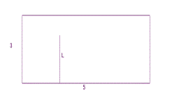
3. Suppose the dart board for our experiment is a 3' by 5' rectangle
and when the dart lands we report the distance of the dart to the
5' side with the random variable L. [See Figure I.18] 
a. Find the point probability density for L at 1.
b. Find the point probability density for L at $A$ with 0 < $A$ < 3.
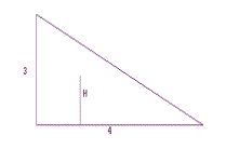
4. Suppose the dart board is a right triangle with legs
3' and 4' and when the dart lands we report the distance of the dart to
the 4' side with the random variable H. [See Figure I.19] 
a. Find the point probability density for H at .1.
b. Find the point probability density for H at $A$ with 0 < $A$ < 3.
5. Suppose X is a random variable which takes values in the interval
[0,2] and that for each of the following definitions of F, F($A$) gives
the probability that X $A$ where 0<$A$<2.
i. Find the (point) probability density of the distribution
for X at 1.
ii. Find the (point) probability density of the distribution
for X at $A$ where 0 < $A$ < 2.
a. F(A) = .5 A. b. F(A) = 1/4 A 2.
c. F(A) = A2 - 3/2 A.
d. F(A) = 1/8 A3 . e. F(A) = 1/16 A4.
6. Suppose F(A) = sin(A) describes the probability that a
random
variable Y is less than or equal to $A$ where 0 < A < π
/2. Using your calculator estimate the point probability density
for Y at π/4 using the intervals [ π/6, π/4]
, [π /4, π/3], and [π /4, π /4 + .1]. Discuss briefly
what you think the
point probability density for Y at π /4 might
be. [See problem 11 in section 0.C.]
7. Suppose that an object is inside a sphere of radius 10 centimeters
and it is equally likely that it is at any point in the sphere. Let $R$ denote
the random variable that measures the distance from the object to the center
of the sphere. [See problem 12 in section 0.C.]
Why is the probability that $R$ <= A with A < 10 given
by A3 /1000? Find a formula for the point probability density
for $R$ at $A$ with 0 <$A$ <10.
8. In Example I.C.1 consider the average probability density for intervals
of the form [x,60] and [60,x]. Discuss the issue of whether there is a
point probability density for $R$ at $A$=60 based on some calculations for
these intervals.
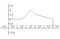
9. Another Darts Board. Suppose the dart board has a shape bounded
by the polygon in Figure *** in the coordinate plane and when the dart
lands we report the first coordinate of the point measuring the distance
of the point to the Y axis with the random variable X.

a. Draw a mapping diagram and sketch of what the
cumulative distribution function F for X might be, based on the figure,
i.e., the function F where F(A) is the probability that $X \le A$.
b. Estimate the point probability density for X at $A$ = 1, 2,
3, and 4..
c. Find the point probability density for X at $A$ with 0 < $A$ < 5.
10. Point Probability Density and The Tangent Problem. Write
a comparison of the treatment of point probability density to the
solution of the tangent problem. Discuss the following statement in your
essay: " The probability density of a random variable X at a point $A$ is
measured by the slope of the line tangent to the graph of the cumulative
distribution function F at the point $(A,F(A))$."
11. Project on Estimation and Archimedes: The Greek mathematician and
scientist Archimedes (287-212 B.C.E.) wrote perhaps the first work to give
a systematic method for estimation. Read On the Measurement of the Circle
where Archimedes estimates pi in Proposition 3. Write a paper describing
the content and method of this work.


 .
.