28th International Conference on Technology in Collegiate Mathematics
ICTCM (logo)
2016
¤
March 12, 2016
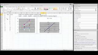
Mapping Diagrams for Complex Variable Functions
Visualized Dynamically with GeoGebra
1:30 p.m. - 2:00 p.m.

Part I
Mapping Diagrams for Real Functions
Complex Arithmetic
Part II
Complex Functions
Part III
Calculus for Complex Functions


Martin Flashman
Professor of Mathematics
Humboldt State University


http://flashman.neocities.org/Presentations/MD.ICTCM.CV.3_12_16.html


5.1 Limits and  Continuity   ¤
Definition:  $\lim_{z \rightarrow z_0} f(z) = L$ means:
Given any $\epsilon>0 $ there is a $\delta> 0$ so
that if $0 <|z-z_0|<\delta$, then $|f(z)- L|<\epsilon$.

Example: $\lim_{z \rightarrow i} z^2 + 2z = -1+2i$ means:
Given any $\epsilon>0 $ there is a $\delta> 0$ so
that if $0 <|z-i|<\delta$, then $|z^2 +2z +1-2i|<\epsilon$.


5.2 The Derivative for Complex Functions    ¤
5.2.1 The Derivative for Powers of z: $f(z) = z^n$.
$$f'(z_0)= \lim_{\Delta z \to 0} \frac{f(z)-f(z_0)}{z-z_0}$$


6.1 Visualizing the integral $∮_C \frac1z dz $. ¤


Thanks for attending¤.

Questions?

The End!


http://flashman.neocities.org/Presentations/MD.ICTCM.CV.3_12_16.html


References:¤

Mapping Diagrams from A(lgebra) B(asics) to C(alculus) and D(ifferential) E(quation)s.
A Reference and Resource Book on Function Visualizations Using Mapping Diagrams

The Sensible Calculus Program