Section OW Other Algebraic Functions
Introduction: The concept of a function can be
applied to have more than two variables interacting. One common
application of the function concept has two, three or "$n$" variables
controlling a single variable: $ f: R^n \to R$.
Another application has a single variable controlling two, three or "$k$" variables.: $ f: R \to R^k$.
Even more complicated is a function that uses two, three, or "$n$"
variables to control two, three, or "$k$" other variables: $ f: R^n \to
R^k$.
The methods for studying multi-variable functions can become quite abstract when a total of more than three variables are involved. In part this is due to the limitations of visualizing more than three variables within visual constraints three dimensional cartesian coordinates.
This limitation for graphical visualization basically restricts the
study of multi-variable functions to $f: R^n \to R^k $ where $n = 2 $
and $k = 1$ or $n=1$ and $k = 2$.
A multi-variable function is
defined by techniques similar to those used to define single real
valued functions of a single variable. The tools for visualizing
these functions beyond the constraints of three dimensional cartesian
geometry to investigate the wide range of related concepts of
continuity, differentiability, and integrability can benefit much from the use of mapping diagrams.
The key idea in visualizing multi-variable functions with mapping diagrams is to have $n+k$ parallel number lines (or axes),"n" lines representing the source (input, controlling or independent) variable values and the other $k$ lines representing the target (output, controlled or dependent) variable values. The function is visualized by arrows that relate points (numbers) on these parallel axes.
Mapping Diagram Definition
Using some dynamic technology with GeoGebra we can see connections between the graph and mapping diagram visualizations.
Connecting Mapping Diagrams and Graphs
Example TMD.0 The First Example.
This example presents a single function using an algebraic formula, a table of data, a graph and a mapping diagram.
You can download and try the worksheet for this section now: Worksheet.VF1.pdf.
Notation for Graphs and Mapping
Diagrams
Subsection VF.TTGM Technology: Tables, Graphs, and Mapping Diagrams
Subsection VF.DTGM Dynamic Technology: Graphs, and Mapping Diagrams
Exercises X.VF: Exercises for Visualizing Functions
OW.FDPC Function Definition by Piecewise Cases
Functions defined by piecewise cases are characterized by partitioning the domain of the function and defining the function value by identifying in what particular subset of the partition a number lies. Wikipedia on piecewise-defined functions.
A very simple example of a function defined by piecewise cases is the function $\chi_3$ where $\chi_3(3) = 1$ and $\chi_3(x) = 0$ for any $x \ne 3$.
[This function $\chi _3$ is described as "the characteristic function of the number $3$."]
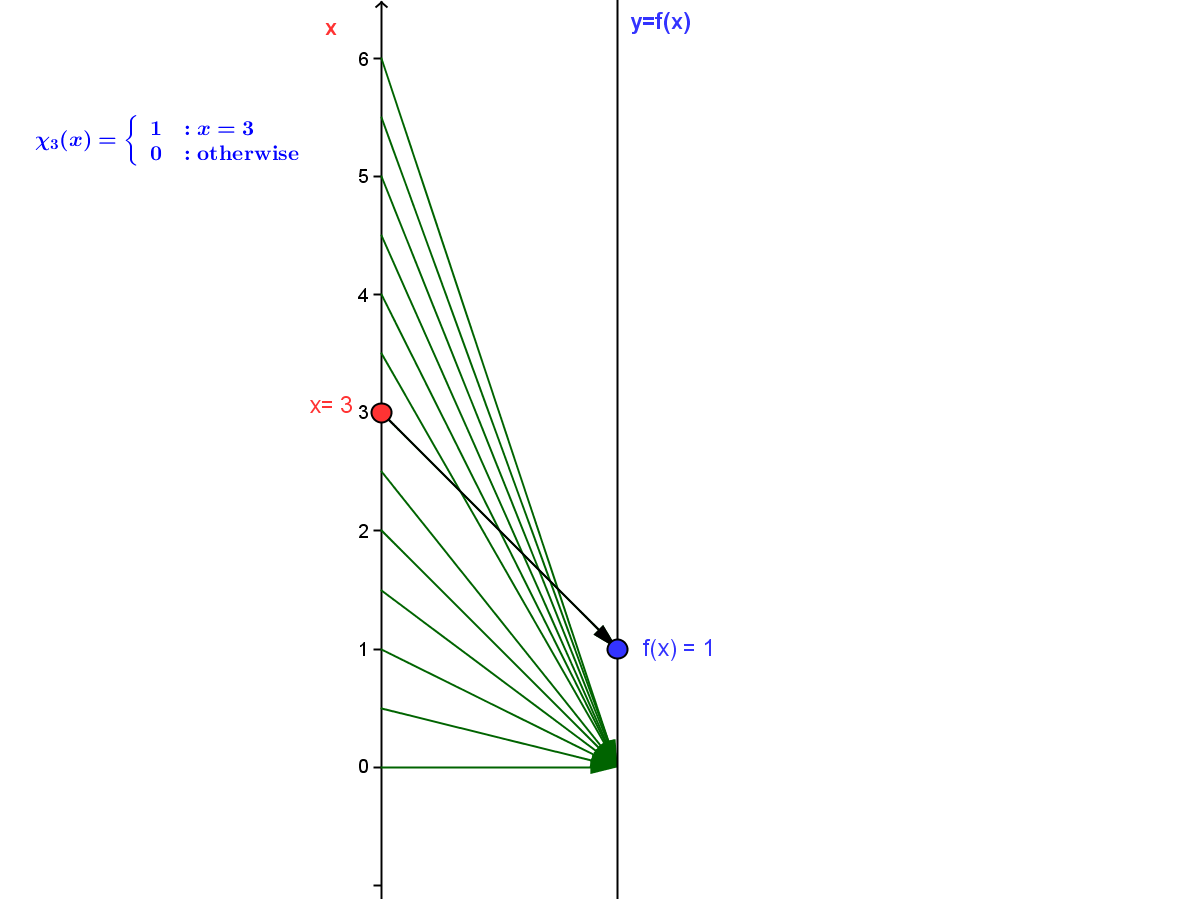
Mapping Diagram for $\chi_3$
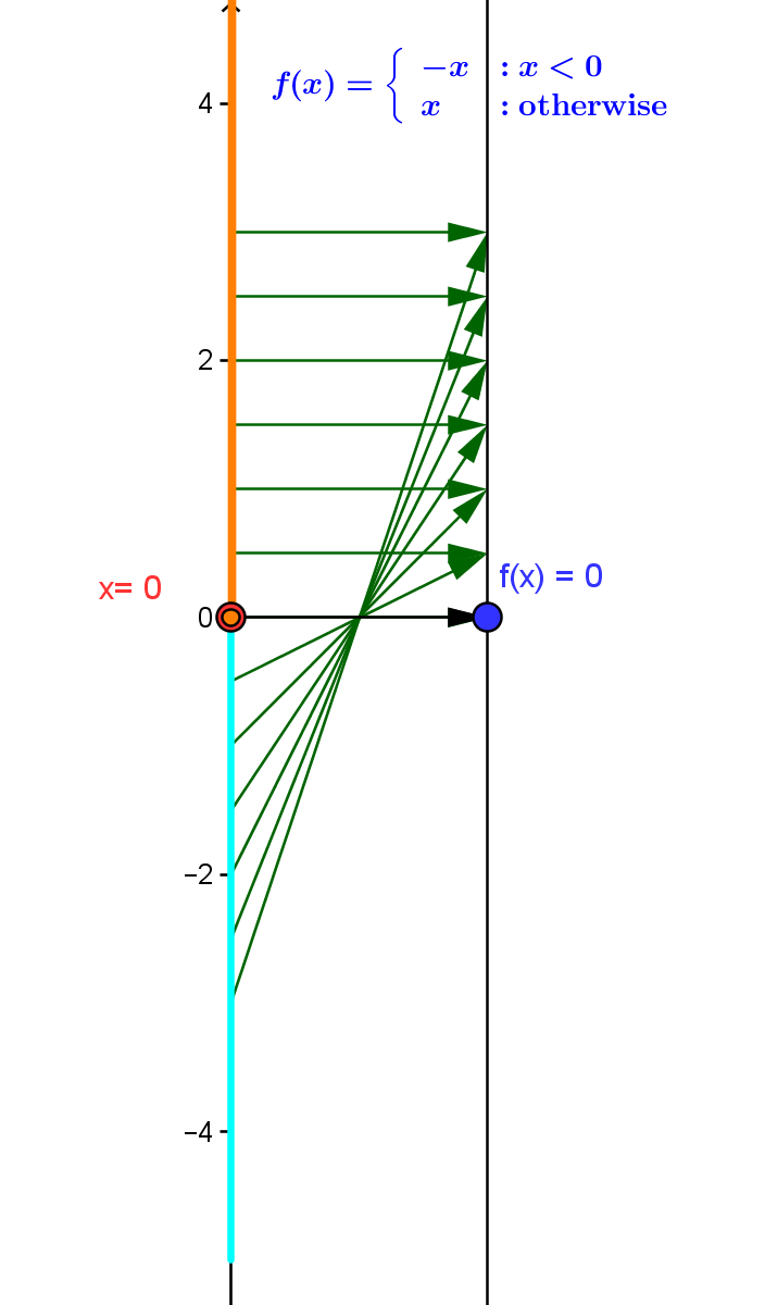
Mapping Diagram for $f(x) = |x|$
OW.FDINV Function Definition by Inversion
We have already discussed inverse functions and mapping diagrams in the section LF.INV on inverses of linear functions. See also Wikipedia on Inverse Functions.
We investigate definition by inversion further by exploring the core positive power functions $P_n(x) = x^n$ and their "inverses. "
Comment: Consider the core power function $P_3$ where $P_3(x) =x^3 $. This function has a unique inverse function which we denote by $InvP_3$ or $P_3 ^{-1}$. It is commonly know as the "cube root" function so $InvP_3(x)= P_3 ^{-1}(x) = \sqrt[3] x$ . The property that defines $invP_3=P_3 ^{-1}$ is that $ P_3(P_3 ^{-1}(x)) = (\sqrt[3] x)^3 = x$ for all numbers $x$. We can also understand this by saying $P_3 ^{-1}(s)$ is defined as the unique number $t$ where $P_3(t) = t^3 =s$.Applications of this method are studied extensively in intermediate algebra (for logarithms) and trigonometry ( for inverse trig functions).
OW.FDImpl
Implicit Function Definition
Functions implicitly defined by an equation are not
mentioned in beginning algebra courses but occur quietly in
the background connections between linear (line) and
quadratic (conic curve) equations and functions. Wikipedia
on Implicit Functions.Comments:
- A very revealing example is given by recognizing an inverse function for the function $f$ is an implicit function for the equation $f(y)-x = 0$.
- A commonly encountered example is given by recognizing
that the function $f(x) = \sqrt{ 1- x^2}$ for $x
\in [-1,1] $ is an implicit function for the
equation $x^2 +y^2 - 1 = 0$.
This example presents a (piecewise) case defined
function $f$, implicitly defined with respect to the
equation $x^2 +y^2 -4 = 0$ with a table of data, a
graph and a mapping diagram.
OW.FDRec Recursive Function Definition
Functions defined recursively (inductively) on subsets of the integers or related subsets of the real numbers are usually not mentioned directly in algebra courses, yet are encountered through experience in these and later courses both with sequences of numbers and of functions. Wikipedia on Recursive Definition of Functions.Examples of recursive functions $f: N \rightarrow R$ include the factorial function defined by $f(0)= 1$ and $f(n+1) = (n+1) \times f(n) $ for all $n > 0$ and the Fibonacci sequence function, defined by $f(0)=0$, $f(1)= 1$ and $f(n+2) = f(n) +f(n+1)$. Both these functions can be visualized by mapping diagrams.
|
Fibonacci Function
|
|
 |
||||||||||||||
| Factorial
Function |
|
 |
Treatment of functions defined by cases and by inverses with their graphical interpretation is common in algebra courses in preparation for calculus.
Functions defined implicitly by equations or recursively are not mentioned much, if at all, before a first course in calculus.
What is missing is a balanced treatment using mapping diagrams to reinforce the function aspect in the visualizations of these other ways to define functions. That will be emphasis of this section. It will provide examples that will help students use the power of the mapping diagram along with the three other tools (equations, tables , and graphs) to understand these other ways to define functions.
You can download a spreadsheet OW.TSS.0.xls with examples of these other ways to define functions.