2015 Joint Mathematics Meetings
  "Revitalizing Complex Analysis"
¤
January 9, 2016
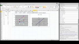
Visualizing Complex Variable Functions with Mapping Diagrams:
Linear Fractional Transformations.

Martin Flashman
Professor of Mathematics
Humboldt State University

http://flashman.neocities.org/Presentations/JMM2016/MD.JMM.CV.1_9_16.3.html


Abstract: Crucial to understanding much about complex variable functions is a sound comprehension of core linear fractional transformations. In a recent undergraduate complex variables course the author used GeoGebra 5.0 to create mapping diagrams for these functions in a three dimensional setting. The diagrams are modeled after mapping diagrams for real variable functions. Several visual features of these functions and their complex integrals will be illustrated that can add to the understanding of these core functions. The diagrams will be available for use over the internet.
Background and References to other work on Mapping Diagrams for real variables ¤


1.1.Background: Mapping Diagrams for Real Functions . ¤


1.1.1 What is a mapping diagram?
Introduction and simple examples from the past: Napiers Logarithm


See: http://www.maa.org/press/periodicals/convergence/logarithms-the-early-history-of-a-familiar-function-john-napier-introduces-logarithms

Logarithms: The Early History of a Familiar Function - John Napier Introduces Logarithms  by Kathleen M. Clark (The Florida State University) and Clemency Montelle (University of Canterbury)
Figure 3. Modern version of Napier's diagram

1.1.2 Real Functions. ¤
Understanding Real Functions: Tables, Mapping Diagrams, and Graphs 


1.2. Real Linear Functions. ¤
Real Linear functions are the key to understanding calculus.
Linear functions are traditionally expressed by an equation like :
$f(x)= mx + b$.
Mapping diagrams for real linear functions have one simple unifying feature- the focus point, determined by the numbers
$m$ and $b$, denoted here by $[m,b]$
.
Mapping Diagrams and Graphs of Real Linear Functions
Visualizing real linear functions using mapping diagrams and graphs.
This is a Java Applet created using GeoGebra from www.geogebra.org - it looks like you don't have Java installed, please go to www.java.com
Notice how points on the graph pair with arrows and points on the mapping diagram.

2.1. Complex Functions

Functions of complex variables can be visualized in a 3 dimensional figure by mapping diagrams between parallel complex planes.
Here are some examples of
linear functions, linear fractional (Moebius), and power functions I have built using GeoGebra .

2.1.1 A complex linear function can be visualized as a mapping from $\mathbb{C}$ to $\mathbb{C}$.¤
Mapping Diagram for Complex Linear Function (using points on circles for sampled domain.)

This example shows a linear function $f(z) = a + bz$ where $a$ and $b \in \mathbb{C}$ on a single complex number $z$ and points on a circle in the domain complex plane.
 

Use the "r" slider to change the radius of the circle in the domain for the mapping diagram.
Move $a$ and $b$ in the plane to change the value of these complex number parameters.
Notes:
  1. When $a=0$ and $b \in \mathbb{R}$ then $f$ is a dilation and the arrows lie on a section of a cone. The vertex of the cone is the focus point with axis orthogonal to the complex planes at $0$.
  2. When $a=0$ and $b = e^{i\Theta} $ then $f$ is a rotation isometry about 0 by $\Theta$ radians and the arrows lie on a section of an hyperboloid of one sheet between circles of equal radii centered at $0$.
  3. When $b = 1$ then $f$ is a translation isometry by $a$ and the arrows lie on a cylinder between circles of equal radii, one on the source centered at the $0$ and the other on the target centered at $a$.
  4. In general one can understand $f$ as a composition of these three types of functions, $f = s_a \circ r_{Arg(b)} \circ m_{|b|}$ where $m_{|b|}(z) = |b|z$ , $r_{Arg(b)}(z) = e^{Arg(b) i} z$, and $s_a(z) = a + z$.


2.1.2 Linear Functions visualized with cones and geodesics.
In the following figure for $f(z) = bz$ the mapping diagram is based on the cone for
$m_{|b|}(z) = |b|z$ as visualized in the previous figure. You can choose either the arrow mapping diagram or a mapping diagram using geodesics between $z$ and $f(z)$ on the cone to visualize $f$.


2.1.3 Complex Mapping Diagram of Linear Function (using points on lines for sampled domain.) ¤
This example shows a linear function $f(z) = a + bz$ where $a$ and $b \in \mathbb{C}$ on a single complex number $z$ and points on a line in the complex plane.


You can move the point $z_#$, change the slider to move the line, and enter a new function.

3.1 Visualizing Complex Linear Fractional Transformations [Moebius Functions] with Mapping Diagrams ¤
This example shows a moebius linear fractional function $f(z) = \frac {a + bz}{c+z}$ where $a$, $b$ and $c \in \mathbb{C}$ on a single complex number $z$. You can move $a,b$,and $c$ in the Graphics window to change the complex parameters for the Moebius function.


The sliders adjust the slope of the lines through $0$ and the radius of the circles centered at $0$ for the mapping diagram arrow source.
Notes:
  1. When $b=c=0$ and $b=1$ then $f$ is complex inversion and the circular based arrows cross on a line above the real axis.
  2. When $a=1$ and $c=0 $ then $f$ is the composition of complex inversion followed by translation by the complex number $b$.
  3. When $a=1$ and $b=0$ then $f$ is a translation isometry by $c$, followed by complex inversion.

3.2 Mapping Diagrams can also connect to the Riemann sphere.¤
The following mapping diagram for a general Moebius function demonstrates the projective connection of the image complex plane to the Riemann sphere.This example shows a $f(z) = \frac {a + bz}{c+ dz}$ where $a$, $b$, $c$ and $d \in \mathbb{C}$ on a single complex number $z$.
To change the complex parameters for the Moebius function y
ou can move $a,b,c$,and $d$ as well as the center of the circle $O$ in the Graphics window  You change the radius $r$ of the circle with the slider.
Notice that if the circle passes through a pole of the function, the image is a line corresponding to a circle on the Riemann Sphere passing through the point at infinity.


4.1 Visualizing the integral $∮_C \frac1z dz $.


5.1 Bonus!? Visualizing Complex Power Functions with Mapping Diagrams ¤


The sliders adjust the height of the second complex plane, the power, n, and the radius of the circle for the mapping diagram arrow source.


Thanks for attending
¤.

Questions?

The End!

http://flashman.neocities.org/Presentations/MD.JMM.CV.1_9_16.html


References:¤

Mapping Diagrams from A(lgebra) B(asics) to C(alculus) and D(ifferential) E(quation)s.
A Reference and Resource Book on Function Visualizations Using Mapping Diagrams

The Sensible Calculus Program