Dec., 2005: This page now requires Internet Explorer 6+MathPlayer
or Mozilla/Firefox/Netscape 7+.Preface: The definition of the derivative articulates a concept used in understanding
rates of change in several different contexts where one variable "controls"
the value of another variable. In chapter IV our examination of differential
equations demonstrated that knowing the derivative (how fast we are traveling
on a highway) can help us determine its primitive function (our location
or change in position as a function of time). In another context, knowing
how fast the rain is falling allows us to find the watershed volume or
water level (change in water volumes or heights) as functions of time.
The problem of solving differential equations was investigated using graphical
tools (tangent fields and integral curves), numerical tools (Euler's method
for estimating the values of solutions with initial conditions- a numerical
integration) and, for a more limited family of differential equations,
symbolically (indefinite integrals).
In finding exactly and estimating functions to solve differential equations
we have seen another concept taking shape to understand change. In somewhat
abstract terms, we want to find the net change in the value of a controlled
(dependent) variable for a given interval of the controlling (independent)
variable. The consolidation (integration) of information about a controlled
variable's rate of change,`{dy}/{dx}=f '(x)`,
with respect to a single controlling variable, x, for the interval
[a,b], leads to the recovery of information about the net
change in the controlled variable's values, `Deltay
=f (b) – f(a)`. This context is common
enough to articulate it more carefully and distinguish it from those already
developed in solving differential equations.
In our study we found that by accumulating estimates of change in a
controlled variable (dy ` ~~ Delta`y) over small intervals of change in the controlling variable (dx
= `Delta`x) we could make reasonable
estimates of the net change in the controlled variable over a longer interval
( [a,b]). In this chapter we will define and begin to study the concept
called the definite integral that captures this procedure of accumulating
estimates and the number estimated by this process.
V. A. A[n Informal] Definition of The Definite
Integral (Euler)
The sums used in Euler's method (Chapter IV.***) to estimate the solution
to a differential equation of the form f '(x) = P(x)
where P was a continuous function had at least two interpretations, one
related to motion and one related to areas.
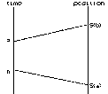
In the motion interpretation these sums estimated the net change in
a moving object's position, S, during the time interval [a,b], i.e.,
S(b) - S(a), based on the model assumption that its velocity at time t
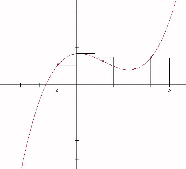
was given by v(t) = S'(t) = P(t). See Figure 1.
Figure 1
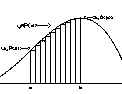
In the geometric interpretation when P(x) > 0 the
sums estimated the area of the region in the coordinate plane enclosed
by the X axis, the lines X = a and X = b, and the graph of
the function P, i.e., the graph of the equation Y = P(x).
See Figure 2. The fact that these sums appear to approach a single number
as their limit and the importance of these sums in a variety of interpretations
has led to the articulation of the mathematical concepts involved.
Figure 2
Overview: The abstraction that has developed from these and other
interpretation of these estimations focuses on the limiting number, called
the definite integral of the function P over the interval [a,b].
As we proceed to give a[n informal] definition of this concept, keep in
mind that we are describing the specific number which is the limit of
these estimating sums. As the number of summands increases the estimating
sums approach a single number which can be interpreted in the two distinct
models using the function P to describe either the velocity of a moving
object or the graph of a function bounding of a planar region. The definition
with which we begin works perfectly well for continuous functions on compact
(closed and bounded) intervals, so we will use it initially to describe
the key properties of the definite integral and its applications. Later
we will explore how the definition we have given can be extended to allow
more general considerations on estimating this number and also to overcome
some more subtle problems with functions that are not continuous (step
functions and functions with vertical asymptotes) or for intervals that
are not compact (bounded, open intervals and unbounded intervals). Using our work in Chapter IV as a guide, we first establish
some notation.
Notation: Suppose that P is a function defined on the interval
[a,b] and N is a positive integer. We will use let dx = `Delta x
=h =(b-a)/N`.
With this established we continue by denoting a by x
0, so a = x 0, and then we let x
1 = a + `Delta`x,
x
2= x 1 + `Delta`x
= a + 2 `Delta`x ,
x
3= x 2 + `Delta`x
= a + 3 `Delta`x .
We continue this notation simply by letting x k
= a + k `Delta`x. Note
that this means that x N = a + N `Delta`x
= b.
Since the numbers x k arose in the context
of Euler's method for solving a differential equation,
we describe
the set {`a = x_0 , x_1 , x_2 , ... , x_N =b`} as an Eulerian partition
of the interval [a,b] with norm or meshdx = `Delta x
=h =(b-a)/N`.
Notes:
1. We have assumed that a<b, so that dx = `Delta`x
= h > 0 and thus `a = x_0 < x_1 < x_2 < ... < x_N =b`.
2. As the size of N increases, the size of `Delta`x
= h approaches 0. Symbolically, as N ` -> oo, Delta x =
h -> 0`.
3. If we had chosen a and b without the presumption that a<b, all
the notation would still make sense, though if b<a then `Delta`x<0
and `b = x_N < x_{N-1} < ... < x_1 < x_0 =a`.
As we have said before, sums were important quantities in estimating
the net change in position and the area in our previous work, so we establish
a shorthand notation for these important numbers as well by letting
`S(P,N) -= P(x_0) Delta x
+ P(x_1) Delta x
+ ... + P(x_{N-1}) Delta x `.
(*)
We'll refer to these sums as the Nth Eulerian sum for
the function P over the interval [a,b] or the Eulerian
sum for short.
More Notes: 1. The Eulerian partition of [a,b]
breaks the interval into N distinct segments (sub- intervals). In the Eulerian
sums we evaluate the function P at the left hand endpoint of each of these
intervals. The left hand endpoint of the first segment is x
0, the left hand endpoint of the second segment is x
1, the left hand endpoint of the third segment is x
2, and the pattern continues with the left hand endpoint of the
kth segment being xk - 1, so that last
summand of S(P,n) evaluates P at the left-hand endpoint of the (last) Nth
segment, namely xN - 1.
2. The Democracy Principle : "What's good for one is good for all."
Essentially the sum is the accumulation of the results of the same
computational process applied to each subinterval: Evaluate P at the left
hand endpoint of the segment, then multiply that result by `Delta`x. This is one of the key principles for all of mathematics!
Historical Comment: The precise definition of the definite integral
has had a long history and as with many mathematical concepts, with its
continued refinement it has gained in abstraction and power. It was Augustin
Cauchy who is generally credited with bringing some precision to these
concepts in the early 19th century, but the development continued to its
generally acknowledged first completion in the mid 19th century by the
German mathematician Georg Friedreich Bernhard Riemann (1826 -1866). Only
in the beginning of the 20th century did the definite integral reach its
full generality with the work of the French mathematician Henri Lebesgue
(1875-1941) on what is now described as the theory of measure. The notion
of the definite integral has continued to grow further even in the 20th
century, demonstrating the vitality of the concept in an ever expanding
world of mathematical studies.
3. As we have seen in Chapter IV, it is sometimes simpler for computational
purposes to use the formula
which results from recognizing the common factor of `Delta`x
in equation *.
4. Although the notation ignores the relation between the number N and
the other subscripts used in denoting the numbers in the partition of [a,b],
don't be fooled into thinking that the partitioning numbers are the same
for different N. For example, for the interval [0,5] the Euler partition
with N = 5 is {0,1,2,3,4,5} so with N= 5 it turns out that xk
= k. But with N=4, the Euler partition is {`0, 5/4, 5/2, 15/4, 5`} or xk
= `(5k)/4`.
The notation ignores the different values of N, but it is important
to recognize this, since it means that data used to compute with N= 5 will
be different from that used to compute with N=4.
If we wish to use data computed when N=5 in the computation of S(P,N)
for other values of N, 5 must be a factor of N. Here is another place where bisection or decimation can come in handy
as a technique for computing that does not discard old information.
5. Our treatment here has emphasized the motion and area
interpretations
of the definite integral, but we should not forget that the
differential
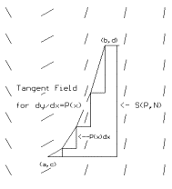
equation tangent field also can be used to visualize these sums. In
particular
we can interpret S(P,N) using a tangent field for the differential
equation `(dy)/(dx) = P(x)` and estimating an integral curve for this
field
with line segments.
See Figure 3.
We can consider this estimate as an approximation for the graph of a
position function s that satisfies the differential equation. Now
locate the points on the estimating curve with first coordinates a
and b. Assume these points have coordinates (a,c) and (b,d). The
interpretation of the sum as the net change in position is now seen as
the accumulation of the step by step vertical changes made by this estimating
curve over the interval [a,b]. Thus we see as well that
`S(P,N) ~~ d - c`
and represents an estimate of the net change in the second coordinates
for an integral curve fitting this field.
Figure 3
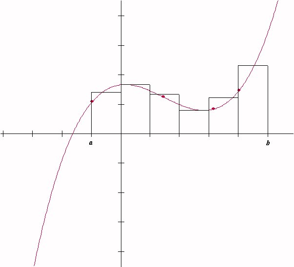
6. The Party Principle: "The more the merrier." By taking N larger, the number of summands increases.
Our experience with the interpretations of motion and area suggest that
the sums will approach a specific number.
This suggests that the more subintervals
and data computed, the closer the sum will come to the limiting value.
Example V.A.1. In this example we consider some specifics in
computing the Euler sums.
Suppose P(x) = 3 x 2 and a = 1 while
b = 5 with N = 4. Then `Delta x
= (5 -1)/4 = 1` and so x 0 = 1 , x 1
= 2, x 2 = 3 , x 3 = 4, and x
4 = 5.
Using N = 40, gives `Delta x = (5 -1)/40
=1/10`. This N decimates the interval with segments of length 0.1 so the
partition is {1, 1.1, 1.2, 1.3, 1.4, ... ,4.8, 4.9, 5} Finding the values
of P at 40 numbers is something best left to some kind of calculating program
or spread sheet. It can also be computed using some clever algebra [1],
but however it is done, the sum `S(P,40)~~120.42`.
Of course much larger values of n would be even more difficult without
the aid of a calculating procedure or better algebra.
Here is a table showing
the results of further computation of S(P,N) in a decimating scheme.
N
`Delta`x
S(P,N)
40
0.1
120.42
400
0.01
123.6402
4000
0.001
123.964002
40000
0.0001
123.99640002
400000
0.00001
123.99964
4000000
0.000001
123.999964
It seems clear from this table that as N gets larger, the values of S(P,N)
get close to 124.
Recall that in Chapter IV we saw in the Fundamental Theorem
of Calculus that
these sums would be approaching F(5)-F(1) for any function
F where F '(x) = P(x) = 3x2.
Using F(x) = x3
we see that the table is not misleading in its values since 53
-13 = 124.
(Informal) Definition: The Definite Integral - Euler: Suppose
P is a function defined on [a,b] and S(P,N) is defined as above. As we
have seen in Chapter IV, it is often the case that when N is very
large the values of S(P,N) approach the number I. In this case we say that
P is (Euler) integrable over the interval [a,b] and we call I the
definite integral of P over the interval [a,b] (or I is the definite
integral of P from a to b). In this situation we denote I by the
following symbols ( due to Liebniz):
I = `int_a^b P dx = int_a^b P(x)dx`
The work of chapter IV suggests two results that we record here with
a brief review of the evidence we have for their being true.
Theorem V.1. (Continuity implies Integrability) If
P is a continuous function on [a,b] then P is integrable.
Theorem V.2 (The Fundamental Theorem
of Calculus - Evaluation Form)
Suppose P is a continuous function on [a,b] and
F is a differentiable function on [a,b] with F '(x) = P(x)
for all x in (a,b). Then
I = ` int_a^b P(x)dx` = F(b) – F(a)
Evidence for Theorems V.1 and V.2:
Motion Interpretation. Consider P as a velocity function
which changes continuously for the time interval [a,b]. We can consider
the sums S(P,N) as the result of selecting the velocity values at a finite
number of points in the time interval, using these velocities to estimate
the change in position for short time intervals, and then accumulating
these estimates for an estimate of the net change in position for an object
moving with velocity P for the time interval [a,b]. Since the velocity
is a continuous function we can perform a thought experiment setting controls
for an object to move with the given velocities. When the object in this
experiment moves we can keep track of its position with the function F.
Its net change in position for the time interval [a,b] will
be the number F(b)-F(a). This is the number that the sums S(P,N)
approach when N is very large.
Cost Interpretation. Consider P as a marginal cost
function
which changes continuously for the production level interval [a,b]. We
can consider
the sums S(P,N) as the result of selecting the marginal cost values at
a finite
number of points in the proction level interval, using these marginal
costs to estimate
the change in cost for short production level intervals, and then
accumulating
these estimates for an estimate of the net change in costs for
production for increasing the production over the interval [a,b]. Since
the marginal cost
is a continuous function we can perform a thought experiment setting
controls
for production to change with the given marginal costs. When production
in this
experiment changes we can keep track of its total costs with the
function F.
Its net change in costs for the production interval [a,b] will
be the number F(b)-F(a). This is the number that the sums S(P,N)
approach when N is very large.
Area Interpretation. When P(x) > 0 for all x between a and b, then the summands of S(P,N) can be thought of as the areas of
rectangles that are accumulated to give an estimate of the area of
the region in the plane bounded by the graph of the function P, the lines
X=a, X=b and the X-axis. Since this region seems well contained by
its continuous boundary, it seems reasonable that we can measure its area,
and thus the sums are approaching this measurement.
This supports Theorem V.1's result on the existence of a limiting
number for the Euler sums.
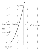
Integral Curve Interpretation:
We form polygonal curves shaped
by lines segments drawn to match the tangent field for the differential
equation `(ds)/(dt) = P(t)`. In particular we can interpret `int_a^b
P(x) dx` using this tangent field and choosing any integral curve
for this field.
We can consider this curve as a graph
of a position function s that satisfies the differential equation. See Figure 5.
Now locate the points on the curve with first coordinates a and
b. These points have coordinates (a,s(a)) and (b,s(b)).
The sums accumulate estimates of changes
in the second coordinates of the endpoint of these curves over the interval
[a,b]. Since P(t) is continuous we can conceive of directing a drawing
instrument to match the differential equation's tangent requirements at
every point of its drawing. This results in drawing polygonal curves shaped
by line segments drawn to match the differential equation `(ds)/(dt) = P(t)`
with an integral curve which the polygonal curves approximate. See Figures
4 and 5. The interpretation of the definite integral as the net change in position
is now seen as the change s(b)-s(a). That is, the definite
integral represents the vertical change in the integral curve over the
interval [a,b]. The net change in the second coordinates of this integral
curve is the number which the sums are approaching.
Figure 4
Figure 5
Example V.A.1. (Cont'd.) With this new notation we can say that
the value of S(P,40) = 120.42 is an estimate for `int_a^b P(x)dx = int_1^5 3x^2 dx`.
Using the Fundamental Theorem of Calculus with F(x) = x
3 we can express our previous conclusion about the value of
this definite integral with the equation
A Little More Notation: As we have seen in chapter IV, the evaluation
of the difference F(b) - F(a)
is both useful and common. For this
reason the older notation for evaluation of a variable has been
extended
to denote this difference by `F(x)| _{x=a}^{x=b} = F(x) |
_a^b = F(b) - F(a)`. So for example in the last
example the work might have omitted the naming
of the function F by displaying F(x) instead as follows:
1. Can we always find an anti-derivative for P as an elementary function?
This would be quite nice, matching the niceness of the derivative
calculus where we have rules that allow us to find the derivative of any
elementary function. Unfortunately this is not the case. Functions as simple
as `sin(x^2)` and ` e^{-x^2}`
do not have antiderivatives that can be expressed as an elementary function.
[The proof of this fact is not easy.] As a result there is no easy way
to find `int_0^1 sin(x^2) dx`
or `int_0^1 e^{-x^2} dx` by applying
Theorem V.2.
2. Is there a geometric interpretation for the definite integral when
the integrand Q is negative on the interval [a,b]?
Yes. If we consider a function Q that is negative
on the interval [a,b], it's opposite,P = -Q,
will be always positive.
See Figure 6. The graph of its opposite,
P, will enclose a region above the X-axis that has the same area as the
region enclosed by the graph of Q, the X-axis, and the lines X = a
and X = b.
But the sums in the estimates for `int_a^b Q(x) dx`
will be opposite the estimates for `int_a^b P(x) dx`.
So we can say that the definite integral for Q will be the opposite
of the integral for P.
Since the integral for P measures
the area of the region, the integral for Q must be the opposite
of the area of the region enclosed by the graph of Q, the
X-axis, and the lines X = a and X =b.
So ... For intervals [a,b] where an integrand Q is negative,`-int_a^b Q(x) dx` is the area
of the region enclosed by the graph of Q, the X-axis, and
the lines X = a and X = b.
Figure 6
Exercises V.A.
Find each of the following definite integrals using the Fundamental
Theorem of Calculus.
`int_0^1 x^2 + 4x^5 dx`
`int_1^2 3x + 5/(x^2) dx`
`int_1^2 1/(x^3) dx`
`int_1^8 x^{1/3} dx`
`int_4^9 -x/2 + sqrt(x) dx`
Estimate the following definite integrals with Euler sums a) with n = 4
, b) with n = 8 and c) n = 100 (using technology). Compare your estimates
with the exact values using problem 1. Explain briefly the quality of your
estimate.
`int_0^1 x^2 + 4x^5 dx`
`int_1^2 3x + 5/(x^2) dx`
`int_1^2 1/(x^3) dx`
`int_1^8 x^{1/3} dx`
`int_4^9 -x/2 + sqrt(x) dx`
Estimate the following definite integrals with Euler sums a) with n = 4
, b) with n = 8 and c) n = 100 (using technology). When possible compare
these estimates with the value obtained for the integral by using the fundamental
theorem of calculus.
`int_0^1 1 + x dx`
`int_0^1 1 + x^2 dx`
`int_0^1 x^3 dx`
`int_0^1 1/(1+x) dx`
`int_1^2 1/x dx`
`int_0^1 1/(1 + x^2) dx`
For each function P on the interval [1,5], give an interpretation for the
sum S(P,4) a) as an area of a region in the plane b) as the net change
in position of a moving object, and c) as the net change in the second
coordinates of two points and a polygonal curve estimating a solution for
a differential equation. Draw any suitable graphs and figures to illustrate
your interpretations.
`P(x) = 2x -1`
`P(x) = 1/x`
`P(x) = x^2`
Give an interpretation with a related visualization for the following integrals
a) as an area of a region in the plane b) as the net change in position
of a moving object, and c) as the net change in the second coordinates
of two points and an integral curve for a differential equation.
`int_0^1 1/(1 + x) dx`
`int_0^1 1/(1 + x^2) dx`
`int_1^2 1/x dx`
Suppose f is a continuous probability density function for a random
variable X on the interval [a,b]. The probability that X will
lie between the numbers A and B with A<B can be estimated by the product
f(A) (B-A).
Discuss the ability to estimate the probability that X will lie between
A and B by the euler sum, S(f , N) for [A,B].
Based on part A) explain why the probability that X lies between A and
B is `int_a^b f(x) dx`.
Suppose an object is moving with its velocity given by v(t)
for time t between a and b. Discuss the relation between
estimating the object's position at time b from its position at
time a using Euler's Method and is equal to `int_a^b v(t) dt`.
Use the fact that
`d/(dt) ln(t) = 1/t` for t >0 to explain why `ln(2) = int_1^2 1/t dt`.
Estimate ln(2) using euler sums for the interval with
N= 4, N= 10, and N= 100. Draw a figure that illustrates this estimation
as an area problem. Discuss the relation of ln(x) for x>1
to a definite integral .
Appendix: Other ways to define the Definite Integral for a continuous
function.
When considering continuous functions over a compact interval, several
alternative definitions can be used to estimate the same number that
we have defined using the left endpoint Euler sums.
Here a some of those
alternatives with figures (to be added still!) illustrating their meaning in terms of both the
motion and the area interpretations of the estimates.
Euler: Let `Delta x = (b - a)/n`
; `x_ k = a + k Delta x`, `k = 0, 1,... n.`
and `S _n(P,n) -= sum _{k=0}^{k = n-1}
P(x _k) Delta x`. Then we define the definite integral by
`int_a^b P(x)d x -= lim _{n -> oo} S_n (P,n)`
Extended Euler: Choose numbers `w_k` so that
`x_{k-1}<= w_k <= x_k ;
k = 1, ..., n` .
Let W = { w 1, w 2, ... ,w n-1,
w n }.
Now we let `S _n
(P,n,W) -= sum _{k=1}^{k = n}
P(w _k) Delta x`. Then we define the definite integral by
`int_a^b P(x)d x -= lim _{n -> oo} S_n (P,n,W)`
Riemann: Start with a partition V of numbers from the interval [a,b], `V = { a = x_0 <=x_1<=x_2<=...<=x_{n-1}<=x_n=b}`.
Let `Delta`x k =
x k - x k-1. Now choose numbers
wk so that
`x_{k-1}<= w_k <= x_k ;
k = 1, ..., n` .
Let W = {w 1, w 2, ... ,w
n-1, w n }and let `Delta`x = mesh of the partition V = max {`Delta`x
k , k = 1 to n}
Now we let `S _n
(P,W) -= sum _{k=1}^{k = n}
P(w _k) Delta x_k`. Then we define the definite integral by
`int_a^b P(x)d x -= lim _{Delta x -> 0} S_n (P,W)`
Without Limits: Let `M_k = `sup `{ P(x), x_{k-1} <= x <= x_k }` [maximum when f is continuous] and
`
m_k =` inf `{ P(x), x_{k-1} <= x <= x_k }` [minimum
when f is continuous].
Using these we continue to define `U_n (P,n) = sum _{k=1}^{k=n} M_k Delta x_k` [The Upper Riemann Sum] and
`L_n (P,n) = sum _{k=1}^{k=n} m_k Delta x_k` [The Lower Riemann Sum]. Then we define the definite integral by
`int_a^b P(x) dx -= ` I, a unique number with the property that for any partition, `L_n (P,n) <=`
I ` <= U_n (P,n)`.
Using an Antiderivative: Suppose G'(x) = P(x) for all x in [a,b]. Then we define the definite integral by `int_a^b P(x) dx -= G(b) - G(a)`.
CAVEAT!
This makes a definition of the Fundamental Theorem so the Fundamental
Theorem must be restated in terms of connecting the definite integral
to some kind of sums!
[1]The
algebra here uses the facts that`1+2+...+(N-1) = ((N-1)N)/2` and `1^2 + 2^2 +...+(N-1)^2 = ((N-1)N(2N-1))/6` to
simplify formula for S(P,N) after the terms `(1 + k 4/N)^2`
have been expanded and the various linear and quadratic terms have been
reorganized: