In this section we will introduce another important tool for understanding differential equations in the context of an initial value problem. In an initial value problem we are given a differential equation together with an initial condition. Our problem is to describe the particular solution function determined by the given information. Unfortunately, it is rarely possible to find an explicit description of the solution function except in the easiest cases. In most of the harder cases the problem becomes that of finding a good estimate for the value of the solution function. One approach, which we will not pursue here, is to make a sketch of the solution using tangent field and integral curve tools (from section IV.D) and then use that sketch to estimate the desired function value. Instead, we will extend the concept of the linear (or differential) estimate to a more general tool.The basis remains knowing the value of the derivative at a particular point.
Review of The Differential: Recall that knowledge of the value of a function and its derivative at a single point can help us approximate the value of the function at a second point. The technique for this approximation was discussed in Chapter III in the section on the differential. There we developed the formula
We also gave geometric, dynamic, and economic interpretations to this approximation. You might review that section quickly now, since we will use those ideas again to find numerical estimates for the solution of a (first order) differential equation with initial condition. This new method based on the differential estimate is called "Euler's method."
Prelude: The following example may seem simple, but if you understand its reasoning you should have little difficulty with its generalization to Euler's method.
EXAMPLE IV.E.1: Suppose f '(x) = x
2 and f (1) = 3. Estimate f (2) using the
differential. Use f '(2) and your estimate of f (2)
to estimate f (3).
Solution: Since 2 = 1 + 1 we can use the differential with a = 1 and h = dx = 1. We use the differential equation f '(x) = x 2 to find that f '(1) = 1 2 = 1.
Thus f (2) = f (1+1) ≈f (1) + f '(1) . 1 = 3 + (1)1 = 4.
Now 3 = 2 +1, so we continue to estimate again, this time finding f '(2) = 2 2 = 4
f (3) = f (2 + 1) ≈ f (2) + f '(2) . 1= f (2) + (4) 1 = f (2) + 4.
It is now time to use the previous estimate of f(2) since we have
no better idea of what f(2) might be. Thus f (3) ≈ 4 + 4 = 8.
Interpretations: [graphical]
The
graphical
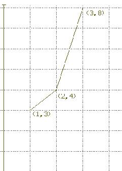
idea of this technique is illustrated in Figure 1. The line with
slope 1 through the point (1,3) gives us the estimate for f
(2). Now at the point (2,4) we use the line with slope 4 to obtain
the estimate for f(3), at the point (3,8). You can think of this
process as going for a walk in the field of tangents determined by
this differential equation. We start the trip at the point (1,3)
and proceed along the line with slope determined by the
differential equation until we come to the point (2,4). Now we use
the differential equation at (2,4) to determine the slope of the
next line and proceed on that line 'til we come to the point (3,8)
where we end our short trip. Instead of walking on the solution
curve, we have been travelling for short segments on lines that
might be tangents to a solution. Note that we could readjust our
lines more frequently thereby taking shorter trips on each segment
before reevaluating the slope. Then we would find our path was
closer to the solution's graph. 
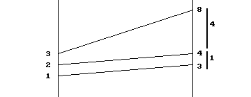
[Motion] The dynamic interpretation of our example is similar. See Figure.2. At time 1 second an object is 3 meters from a point P and its distance from P is increasing at a rate of 1(m/sec). We estimate its position at time 2 to be 4 due to the estimated change in position of 1 meter for the one second of time that has elapsed. Now we find at time 2 seconds that its rate is 4 (m/sec), so we estimate its position at time 3 seconds to be increased 4 meters for the next second of time, giving an estimate for the position at 3 seconds of being 8 meters from P.
[Cost] The economic interpretation of our example is similar. See Figure 2 again. When producing one unit of a product we'll suppose the cost is 3 dollars and its cost is increasing at a rate of 1(dollar/unit). Thus we estimate its total cost for 2 units to be 4 dollars due to the estimated cost of 1 dollar for the additional unit produced. Now we find that at 2 units of production the marginal cost is 4 (dollars/unit), so we estimate the total cost for 3 units of product to be 4 dollars for the next unit produced, giving an estimate for the total cost of producing 3 units as 8 dollars.
Comparison with The Exact Solution: Notice that in using this method the errors of approximation are compounded as we make approximations based on approximations. The exact solution of this differential equation is found easily since $\int x^2 dx = 1/3 x^3 + C$.
Because $3 = f (1) = 1/3 (1)^3 + C$ we have that $C = 8/3$. Thus $f (2) = 1/3(2^3) + 8/3 = 16/3 ≈ 5.333$ and $f (3) = 1/3(3^3) + 8/3 = 35/3 ≈ 11.667$ .
In each case we underestimated the precise value. Can you explain why we should have expected an underestimate from the nature of f '(x)? [Hint: What about the concavity of the graphical interpretation of a solution? What can you say about the acceleration in the dynamic interpretation of a solution?]
If we choose a smaller h at each step, the approximation will be
better, but then we will need to process more steps to arrive at
an estimate for f(2).
Here are the details with $dx = h =
.1$ for estimating f (1.5). [From our exact solution, f
(1.5)= (1.5) 3 /3 + 8/3 = 91/24 ≈ 3.7916667]. You can complete this example to estimate f (2) and f
(3) yourself.
Table 1 shows one way to organize the
information to estimate $f(2)$. Table 2 shows a GeoGebra spreadsheet (downloadable) for the computations using $dx =h= 0.1$ through to $x=3$ and beyond.
[Here is a link for a spreadsheet
you can use to complete this example yourself.]
|
|
Euler's Method: What is the generalization of this method? It is called Euler's method. As it is described below, keep in mind the examples we have just completed.
Step 1. First, suppose that we are given f (x 0) = y 0 and we want to estimate a solution to the differential equation f '(x) = P(x,y) where P(x,y) indicates a number that depends (possibly) on both the values of x and y. [In other words P(x,y) is a function of the two variables x and y. You might think of x as time and y as position in the dynamic interpretation so that we have a context where the velocity is determined by time and position. In the economic interpretation you might think of x as units of production and as y the total cost of production so that we have the marginal cost determined by level of production and current total cost.]
Step 2. We choose a value for h = dx and then let x 1 = x 0 + h.
Step 3. Now we estimate f (x 1)
by y 1= y 0 + P(x
0 , y 0) . h.

We continue by letting x 2 = x 1 + h [= x 0 + 2h] and estimate f (x 2) by y2 = y1 + P(x1,y1) . h.
In general (see Figure IV.E.4) we let
and estimate f (x k+1) by
If x 0 = a and x n
= b then we have that f (b) is estimated by y
n found after n applications of this method.
Since $b = x_n= x_0 + n*h = a + n*h$, if we wish to use this
method to estimate f (b) starting from f (a)
in n steps of equal length, then we use $h = (b-a)/n$.
Here is another example to help you understand this further.
Example IV.E.2. Suppose f (1) = 5 and dy/dx = y - x. Estimate f (3) in 4 steps using Euler's method.
Solution: Linking this example to the notation of the previous discussion, we have
So we set $dx = h = (b - a)/n = (3 - 1) /4 = 1/2 $. Table 2 summarizes the computations for y 1 through y 4 which will be the estimate for f(3). Keep in mind that y k+1 = y k + P(x k,y k) . h.
Thus we estimate the value of f (3) with y 4 = 19.1875 .
Table 3
|
Table 4 using GeoGebra
|
|
|
Here is an opportunity for a programmable calculator, computer
program or spreadsheet to demonstrate its labor saving power as
well as the power of Euler's method. To give a fairly accurate
estimate of the value of f (b) you will want to
work with a large number of steps.
Here is a downloadable GeoGebra applet showing spreadsheets, mapping
diagrams, and tangent (slope) fields together to illustrate some of the
power that Euler's method contributes to making sense of estimating
solutions to an initial value problem.
|
|
[You can also use a spreadsheet which can be downlowded here.]
We'll discuss the accuracy of Euler's method for some
cases in the next section.
Appendix IV.Y has two sample programs
written in BASIC that illustrate the simplicity of Euler's method
and how easily the method's algorithm can be translated into computer instructions.
For the differential equations in problems 1-4, assume y(1) = 2.
(a) Estimate the value of y(3) using Euler's method with n = 4.
Solve the differential equation algebraically and graph the
solution.
Check your results with Sage or GeoGebra. [Remember that $dx = h = (b -
a)/n$.]
(b) Draw a graph of the lines in the tangent plane used in Euler's estimation. Compare the estimate with the exact solution. Based on the concavity of the graph explain the quality of the error in your estimate.
(c) Draw a mapping figure that illustrates the dynamic or the
economic interpretations of Euler's method for your work.
Discuss the interpretation of y'' and how it affects the quality
of your estimates.
| 1. y' = .2 x 3 | 2. y' = x - 1 |
| 3. dy/dx = .5 x | 4. dy/dx = .5 x 2 + 1 |
| 5. y' = 1/x $x \ne 0$ | 6. y' = 1/(1+x) $x\ne-1$ |
| 7. y' = 1/(x 2+1) | 8. y' = x/(x 2 + 1) |
| 9. dy/dt = 2y | 10. dy/dt = -y |
| 11. y' = -2y + x | 12. y' = -2x + y |
| 13. y' = 1/y $y \ne 0$ | 14. y' = 2/(1+y) $y\ne-1$ |
| 15. dy/dx = x 2 + y 2 | 16. dy/dt = 1 /(t 2 + y 2) |
| 17. y' = -x/y $y \ne 0$ | 18. y' = -y/x $x \ne 0$ |
Euler's method can be extended and generalized in many ways. In problems 22-28 we explore extending it to estimate solutions to second order differential equations.
26-28. Problems 23-25 used 4 steps to estimate y(4). Use the same ideas to estimate the solution to those problems with 8 steps.