Graphs and Motion: Secant and Tangent Lines.
It is
commonly presumed that an object moving on a straight line can be in
only one place for a given time, so its position, $s$, is a function
of time, $t$. Two points, $(a, s(a))$ and $(x, s(x))$, on the graph
of this position function report information about two states or
circumstances for the object.
See Figure I.B.6.
The first coordinate of the point gives the time value, $t$, for the
state while the second coordinate gives its position value, $s$. The
change in position between the two states, $\Delta s$, is the change
in the second coordinates of the points, while the change in time,
$\Delta t$, is the change in the first coordinates of the points.
Thus the average velocity determined by the two states,
$\overline{v_a} (x) =\frac {\Delta s} {\Delta t}$ corresponds to the
slope of the non-vertical line determined by the two points. On the
graph of the position function, the slope of the secant line,
$\overline {m_a(x)}$ , determined by the points $(a,s(a))$ and
$(x,s(x))$ uses the same computations used to determine the average
velocity over the time interval between $a$ and $x$. Thus we have
$\overline{v_a} (x) =\frac {s(x)-s(a)} {x-a} =\overline {m_a(x)}$ .
Figure I.B.6
Now our analysis so far
of average velocity and instantaneous velocity has suggested that as $x
\rightarrow a$, the average velocity determined by $x$ and $a$
approaches the instantaneous velocity at
time $a$, i.e.,
$\overline{v_a} (x) \rightarrow v(a)$. Meanwhile our work in Chapter
I.A suggested that the slope of the
secant lines determined by $x$ and $a$ approaches the slope of the
line tangent to the curve that graphs the position function. i.e.
$\overline{m_a} (x) \rightarrow m_{tan}(a)$.
Putting all this together gives us the conclusion that the
numerical value of the instantaneous velocity at time $a$ is precisely the
same as the slope of the line tangent
to the graph of the position function at the point $(a, s(a))$.
Positive velocity is represented by a tangent line with positive slope, going
"uphill" on the graph. while a negative velocity is seen as a tangent line with negative slope, going
"downhill" on the graph. Greater speeds are seen as steeper lines. These relations
can be reversed as well so that a tangent
(or secant) line to the graph of the position function and its slope can be
interpreted to give information about the velocity of a moving object. The
following example and discussion shows more of the connection between the
instantaneous velocity and the slope of a tangent to the position function
graph.
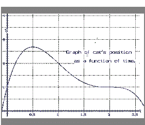
 |
| Figure I.B.7 |
Example I.B.5: Suppose the graph in Figure I.B.7 is the position
function of a cat moving in a narrow chamber with its distance measured
in meters from the door at one end of the chamber. Based on the graph,
estimate the cat's velocity at time 1 second and time 2 seconds.
Estimate the time(s) at which the cat turned around.
Discussion: To estimate velocity based on the given graphical
information about the cat's position, we consider the slopes of the
lines tangent to the graph as measuring instantaneous velocities.
Looking at the point on the graph with first coordinate 1 and estimating
the slope of a line tangent to the graph at that point gives an
estimate of the instantaneous velocity at time 1.
If you draw the tangent line at the point with first coordinate 1, you
will see a line that has a slope of about -2, so we estimate the
cat's velocity as -2 meters per second.
Similarly we estimate the velocity at time 2 by estimating the slope of
the tangent line at the point on the graph with first coordinate 2. This
tangent line seems to be horizontal, so the slope would be 0, meaning a
0 velocity. So the cat appears to be stopped at time 2.
When the cat turned around its position function will change from increasing in value to decreasing or vice versa.
Also its velocity will reverse in sign, and so too will the sign of the
slope of the corresponding tangent line to the graph. Furthermore, for
that instant- when the cat turns around- it will appear to be standing
still. Based on all these criteria we estimate that the cat turned
around approximately when t =.5 since at that point the graph
"turns around," the tangent line slopes change from being positive to
being negative, and the slope of the tangent line at this point appears
to be 0.
Martin
Flashman, Feb. 2, 2014. Created with GeoGebra

