Chapter I: Introduction to The Derivative
(Revised Draft Version 5-27-2014)
© 2005 M. Flashman
| How
do we come to understand Mathematics:
The
discussion of how we can best arrive at
mathematical understanding has certainly
been around for thousands of years.
Current discussions of pedagogy (the art
of instruction) focus attention on the
learner developing understanding of
concepts and techniques through a
mixture of investigations, guided
experiences, and problem solving. When
possible we will try to build an
understanding of calculus concepts on
your prior physical and mathematical
experiences and familiarity with aspects
of common phenomena. |
|
Preface: In this chapter
we begin exploring one of the key concepts of the
calculus, called the derivative. Though the
definition of the derivative in a mathematical
setting is primarily a matter of numbers and
functions, the derivative is important for
its use in various applications that employ
the numerical and symbolic power of mathematics to
study change. These applications have become
important interpretations of the derivative
concept, while providing powerful analytic tools for
the construction of mathematical models. The
interpretations suggest and confirm the truth
of mathematical results when the mathematics fits
well with the experience of the interpretation. This
symbiotic relation of mathematical abstractions with
"real world" interpretations may be a reason for the
unusual success mathematics has had in assisting
scientific studies in so many disciplines. We start
with some key motivation for the derivative
concept. |
In Section A we examine the geometric problem of
describing lines that are tangent to a curve. This
problem should be familiar to you already from Chapter 0.B3,
though previously we considered it using only algebra.
Next we'll turn our attention in Section B to the physics
problem of describing the velocity of an object
moving along a straight line. These two problems have been key
models in the historical development of the calculus.
In
Section C, we'll consider models from probability and
economics (also considered in Chapter 0) which in the
19 th and 20 th centuries have provided
more applications for the calculus outside of the traditional
physical and natural sciences. Further examples and
applications will be found in the exercises illustrating the
importance of the study of change.With these
motivating interpretations it should become apparent that
there is a common mathematical concept used to analyze
each of these models.
The
mathematical abstraction of that common concept leads to the
definition of the derivative in Section D. This
concept has two key aspects, as a number and also as a
function . The definition, its initial application to
"finding the derivative," and other basic concepts in the
study of the derivative will round out this chapter. Procedures
for finding the derivative of function based primarily on
the function's algebraic - symbolic character provide the
first example of a calculus, a calculus for finding
derivatives.
What
lies beyond this chapter: More details of the calculus
of derivatives will be covered in Chapter II. We'll return to
an examination of some traditional applications of the
derivative calculus in Chapter III. In Chapter IV we will
reverse our investigations and examine how information about a
derivative controls the possibilities for related "primitive"
functions. Information about the derivative is usually
presented in the form of derivative (or differential)
equations. Trying to solve these equations provides a sensible
transition to the second key concept of the calculus, the integral,
which, like the derivative, is also both a number and a
function. But for now we can put this second concept aside and
proceed to discuss motivating interpretations for the
derivative.
I. A. [Motivation] Finding the Slope of a Tangent
Line
The
Tangent Problem Again: We are interested in finding the
slope of a line that is tangent to a given
curve at a specific point on that curve. In Chapter 0.B3
we considered the curve with equation $Y = X^2$ and used
the geometric characterization that a tangent line will meet
the curve at only one point to investigate this problem.
Algebra for the equations of the curve and the tangent line
led us to conclude there was only one possible slope for the
tangent line. our work showed that the slope depended only on
the first coordinate of the point. In fact, for the point on
the curve with coordinates (a,a2 )
we found that the slope of the tangent line had to be 2a.
In this section we will follow a different approach to find
the slope of the tangent line. Instead of finding the slope
using algebra alone, we will begin by estimating the
value of this slope, combining algebra with our common sense
of what it means to be close.
|
X
|
Y
|
Slope of Secant =$\frac
{Y-9}{X-3}$
|
|
0
|
0
|
3
|
|
1
|
1
|
4
|
|
2
|
4
|
5
|
|
4
|
16
|
7
|
|
5
|
25
|
8
|
|
6
|
36
|
9
|
Estimating
(the slope of) the tangent line: Our estimates will
depend on examining lines that are close to the
tangent line. One difficulty in our analysis of the tangent
problem is that we have not said precisely what a tangent line
is. The word "close" is also imprecise. We will continue our
investigations without resolving these issues here. The more
experience one has investigating a concept, the more clear its
meaning can become. Articulation of a careful definition
for "tangent" will make more sense later, based on greater
experience .
Example
I.A.1. Estimation and analysis for
$Y = X^2$:
Let's reconsider the question treated in Chapter 0.B.3 of
finding a lin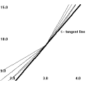 e tangent to the
graph of $Y = X^2$ at the point (3,9). We
call a line that passes through two (or more) distinct
points on a curve a secant
line of the curve. As Figure 1 illustrates,
there are many secant lines to the graph of $Y = X^2$
that pass through the point (3,9). Each of these secant lines
is determined by the first coordinate of a point on the graph
of $Y = X^2$ other than (3,9). So using the
first coordinates 0, 1, 2, 4, 5, and 6 we have different
secant lines determined by the points (0,0), (1,1), (2,4),
(4,16), (5,25), and (6,36). A glance again at Figure 1
should help in understanding that the lines determined
by (2,4) and (4,16) are better
approximations for the tangent line than
the other lines in the figure.
Determining
the slopes of secant lines provides a numerical approach
to finding the slope of the tangent line (previously
discovered to be 6 in Example 0.B.***). In Table 1 we give
these points and the slopes of the secant lines they determine
with the point (3,9) using the formula $\frac {Y-9}{X-3}$.
This table also helps in understanding that the slopes
determined by using (2,4) and (4,16) are better
approximations for the slope of the tangent line than
the other slopes in the table.
It seems
likely from both the visual and numerical views that to obtain
even better estimates of the tangent line and its slope we
should investigate secant lines determined by points (x,
x2) with the first coordinate x
closer to 3. The graphing at this stage can become a little
awkward because of scaling. When x is very close
to 3 the secant line on most graphing devices is almost
indistinguishable from the graph of the function. For this
reason we'll continue the analysis numerically. (Exercises
pursuing the graphical idea of closeness are better explored
further individually with some kind of graphing utility. See
the exercises at the end of this section.)
$x$
|
$x^2$
|
$\bar{m}(x)$
|
|
2.9
|
8.41
|
5.9
|
|
2.99
|
8.9401
|
5.99
|
|
2.999
|
8.994001
|
5.999
|
|
3.1
|
9.61
|
6.1
|
|
3.01
|
9.0601
|
6.01
|
|
3.001
|
9.006001
|
6.001
|
Notation:
The slope of the secant line determined by the number x
will be denoted here with the symbol $\bar{m}(x)$.
Table ***
displays more slopes of secant lines for Example I.A.1, taken
with first coordinates much closer to 3. The pattern in this
chart should be clear. The slope of each secant line is
exactly 3 more than the number x. This pattern is not
by chance. The slope of a secant line determined by the points
(x, x 2) and (3,9) where x is
not equal to 3 is determined algebraically
:
$\bar{m}(x)= \frac {x^2-9}{x-3} = \frac {(x+3)(x-3)}{x-3}
= x+3$.
Thus,
when x is not equal to 3, the slope of the secant
line determined by x is x+3. See Figure
2. When x is close to 3, the slope of the
corresponding secant line, x + 3, will be close to the
slope of the tangent line. But in this situation when x
is close to 3, the number x + 3 is certainly close to
6. Therefore, we can conclude that the slope of the
tangent line at (3,9) must be 6.
Comment:
At this stage there are two ways to think of the use of
the number represented by "x." First, consider a
number, x, as close to (but not equal to) 3 as
you can imagine. For this x, the slope of the secant
line is $\bar{m}(x)= x+3$, which is very close to
6. We'll describe this way of thinking of the estimation as a
static viewpoint, because the number x is
considered fixed.
A second
way to think of this situation is that we are progressively choosing
values for x closer and closer to (but never equal
to) 3. For these x's, the slopes of the
corresponding secant lines, $\bar{m}(x)$,
which could be computed individually using the expression x
+ 3, are closer and closer to the number 6. We'll describe
this way of thinking of the estimation as a dynamic
viewpoint because the number x is considered
changing, varying close to 3.
Notation:
There are some important notation conventions and linguistic
expressions that have developed over hundreds of years to
represent the kind of analysis just made. We discuss now two
ways that will be used throughout the text and are common in
mathematics today.
First, it
is common to write $x \approx 3$ to represent a statement that
x is close (is approximately equal) to 3. In
using this notation we also will allow x to equal 3
and will state explicitly when we exclude that possibility.
With this notation we can express the static viewpoint of our
analysis. We supposed $x \approx 3$ with $x \ne
3$ and found the slope of the corresponding secant
line, $\bar{m}(x) \approx 6$.
A second
very important notation represents either the static or
dynamic viewpoint of estimation with an arrow. With this
notation we write $x \rightarrow 3$ for
the statement that x is close to 3, or that we
are considering x taken closer and closer to 3,
or that x approaches 3. It is usually
presumed that $x \ne 3$, but at times it
is convenient to allow this notation to include the
possibility that the number x may equal 3.
We can
express either the static or the dynamic viewpoint of our
tangent line analysis with this notation. We supposed that $x
\rightarrow 3$ with $x \ne 3$ and algebraically simplified the
slope(s) of the corresponding secant line(s), making it easier
to see that the slope(s), $\bar{m}(x) \rightarrow
6$.
Include
a
picture of the letter $\bar{m}(x)$
in a car approaching a wall labelled 6, with
the letter $x$ on a clock hand approaching
the number 3.
|
|
Review
of Analysis: We have found a method for approximating
the slope of the desired tangent line. We analyzed the slopes
of secant lines, $\bar{m}(x)$, which were controlled by the
choice of numbers for x, the first coordinate of
another point on the graph of $Y=X^2$. When $x
\rightarrow 3$, with $x \ne 3$, by simplifying
algebraically we found that $\bar{m}(x) \rightarrow 6$.
Since when $x \rightarrow 3$ the slopes of secant lines are
better estimates for the slope of the tangent line, we
concluded the slope of the tangent line must be 6.
Generalization:
Frequently a single example has enough of
the basic idea of a solution to a problem
that it can be used as a template to
organize a more general analysis, either
as a computation or an argument. When the
example has dealt with a specific number,
say 3, and the more general analysis
replaces that specific number with a
general number represented symbolically,
for instance using the letter a,
we say we have generalized the example
from the specific number, 3, to any real
number, a.
|
Example I.A.2: Generalization for $Y = X^2$
.
We continue our estimation analysis to find the slope of the
line tangent to the graph of $Y = X^2$
at a
generic point with coordinates $(a, a^2)$
. We
consider the slope of a secant line formed by this point and
the point $(x,x^2)$
which we again
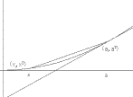 denote $\bar
m (x)$. See Figure 5.
Using
algebra we simplify (since x is not equal to a)
to find $\bar{m}(x)= \frac {x^2-a^2}{x-a} = \frac
{(x+a)(x-a)}{x-a} = x+a$.
When $x
\rightarrow a, x \ne a$, it should make sense now
that $x + a \rightarrow 2a$ and thus $\bar {m}(x)
\rightarrow 2a$.
Therefore,
since when $ x \rightarrow a$ the slopes of the secant
lines improve as estimates for the slope of the tangent line,
the slope of the tangent line at the point with coordinates $(a,
a^2)$ must be 2a.
Comment:
The technique of estimation has become one of the most
effective tools for organizing the study of the tangent
problem. It is not clear when the precise exposition of the
method was first made, but it is certain that the concepts
used in this technique were being developed by many
individuals prior to the work of Newton and Leibniz. Perhaps
it was the blending of these ideas with algebra that began to
yield results in a more systematic fashion, raising
expectations in those days of achieving a more systematic
solution to many other problems as well.
The next
few examples illustrate some of the power and ease that the
interaction of algebra with the analysis of estimation brings
to solving tangent problems.
Example
I.A.3. Find an equation for the line tangent to the
graph of the equation $Y = 3X^2 - X + 1$ at the point
$(1,3)$.
Solution:
We find the slope of the required line using the
estimation method of the last examples. Let $\bar{m}(x)$
denote the slope of a secant line for the curve that passes
through the point $(1, 3)$ and the point on the graph with
coordinates $(x, 3x^2 - x + 1)$. Simple algebra now
shows that when $x \ne 1$, $\bar{m}(x) =\frac {(3x^2 -x
+1)-3}{x-1} =\frac {(3x+2)(x-1)}{x-1}=3x+2 $. Thus when $ x
\rightarrow 1$ with $x \ne 1$, $\bar{m}(x)=3x+2 \rightarrow
5$, so the slope of the tangent line
must be 5. Using the point slope formula we conclude by
finding an equation for the tangent line: $Y = 5
(X - 1) + 3$.
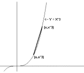
Example
I.A.4. Find the slope of the line tangent to the graph
of $Y = X^3$ at the point $(a,a^3)$.
Solution:
We find the slope of the required line again using the
estimation method. Let $\bar{m}(x)$
denote the slope of a secant line for the curve that passes
through the point $(a,a^3)$ and the point $(x,
x^3)$. [See Figure 1.7.] Simple algebra now shows that when
$x \ne a$, $\bar{m}(x)
= \frac{x^3-a^3}{x-a} = \frac
{(x^2+ax+a^2)(x-a)}{x-a}=x^2 +ax+a^2$
Thus when $x \rightarrow a$ with $x \ne a$, $\bar{m}(x)= x^2+ax+a^2
\rightarrow 3a^2$, so the slope of
the tangent line must be $3a^2$.
Comment: Notice that the slope in this last example is
a non-negative number for any a. Based on the sketch
of the graph of $Y=X^3$, can you explain why this is so?
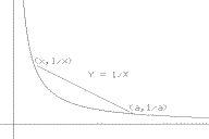
Example
I.A.5. Find the slope of the line tangent to the graph
of $Y=\frac 1X$ at the point $(a, \frac 1a)$ where $a \ne 0$.
Solution:
Again we use the method of estimation of the last
examples. Let $\bar{m}(x)$
denote the slope of a secant line for the curve that passes
through the point $(a,\frac 1a)$ and the point $(x,\frac 1x)$.
[See Figure 8.] Simple algebra now shows that when
$x \ne a$ and $x$ and $a \ne 0$, $\bar{m}(x) = \frac{\frac 1x - \frac 1a}{x-a}=
\frac{\frac {a-x}{xa}}{x-a}= \frac{a-x}{x-a} \frac 1 {xa}
= -\frac1{xa}$.
Thus when
$x \rightarrow a$ and $x$ and $a \ne 0$, $\bar{m}(x) = -\frac 1{xa}
\rightarrow -\frac 1{a^2} $, so the
slope of the tangent line must be $-\frac 1{a^2}$.
Comments:
Notice that the slope in this last example is always
a negative number for any $a$. Based on
the sketch of the graph of $Y = \frac 1X$, can you explain why
this is so?
Compare
the last two examples. Describe the relationship of the sign
of the slope of the tangent line and the graph of the
equation?
Tool for Estimating
Tangent Line Slopes and Instantaneous Velocity (opens in new window)
Exercises I.A. For the
equations in problems 1 through 7, use estimation analysis to
find the slope and an equation of the line tangent to the
graph of the equation at the indicated point.
- $Y = X^2 - X$ ; a)
(1,0)
b)
(-1,2)
c) $(a, a^2 -a)$.
- $Y = 2X^2 - 3X + 1$ ; a)
(1,0)
b) (-1, 6)
c) $(s, 2s^2 - 3s +1)$.
- $Y = X^3 -
X$;
a)
(1,0)
b)
(-1,0)
c) $(a, a^3 - a)$.
- $Y = X^3 - X^2$; a)
(1,0)
b) (-1, -2) c)
$(t, t^3 - t^2)$.
- $Y =
X^4$;
a)
(1,1)
b)
(2,16) c)
$(a,a^4)$.
- $Y = \frac 1{X^2}$, $X \ne 0$
; a)
(2,.25) b) $(a,
\frac 1{a^2})$.
- $Y=\sqrt X $, $X \gt 0$ ; a)
(9,3)
b) $(a,\sqrt a)$.
- For each of the following, use your calculator to
estimate the slope of the line tangent to the graph of
this equation at (0,0) with secant lines when $x = 0.2,
0.1, 0.05, -0.2, -0.1,$ and $-.05$. Discuss briefly what
you think the slope of the tangent might be.
a) $Y = \sin(X)$.
b) $Y = \tan(X)$.
- Use a graphing utility to sketch graphs of $Y
= X^2$ with the secant lines determined by the point (3,9)
with $x = 2.9, 2.99, 2.999, 3.1, 3.01$, and $3.001$.
Each of these should use a different viewing window to
allow the two points to be visible easily. Comment on the
relation of the curve to the secant lines.
- For each of the following equations use your
calculator to estimate the slope of the tangent line at
$(0,1)$ using a secant line when $x=0.001$.
a) $Y = 2^x$
b) $Y = 3^x$ c)$Y =
(0.5)^x$ d) $Y = (\frac 13)^x$
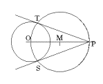 Tangents constructed from
given points not on a curve. One of the traditional
problems for tangents and circles is to construct tangent
lines to a circle through a point given outside of the
circle. See Figure 7. The construction from the point P to
the circle with center O finds the midpoint M of the
segment $\bar{OP}$ and then constructs the circle with
radius $\bar{OM}$ and center $M$. The points where the two
circles meet are $T$ and $S$, and the lines $TM$ and $SM$
are both tangent to the circle.
The next problems ask you to solve comparable problems for
some other curves.
-
 Use
the result of Example I.A.2 to find equations for any
lines that are tangent to the graph of $Y = X^2$
and pass through the point $(3,5)$.
- Use the result of Example I.A.4 find equations for
any lines that are tangent to the graph of $Y =
X^3$ and pass through the point $(2,1)$.
- Use the result of Example I.A.5 to find equations
for any lines that are tangent to the graph of $Y =\frac 1X$
and pass through a) $(1,\frac 34)$
; b) $(1,\frac12)$.
- Find the X-intercept of the line that is tangent to
the graph of $Y = X^2 - 2$ and passes through
the point $(2,2)$.
Normals to Curves: The following exercises explore some
properties of normal lines.
- Find the equation for the normal line to the parabola $Y=X^2$
at $(a, a^2)$.
- Find the equation for the normal line to the
hyperbola $Y=\frac 1X$ at the point $(a, \frac 1a)$, $a
\ne 0$.
- Tangents and the vertex of a parabola.
Consider the parabolic graph of the function $y=f(x) =
x^2- 4x +2$. Find the slope of the tangent at the point
$(a, a^2 -4a +2)$. Discuss why the slope of
the tangent line at the vertex of a parabola determined by
a quadratic function is 0. Use this fact to
find the vertex of the parabola with equation $y=f(x) =
x^2- 4x +2$.
Generalize this example to show the vertex of a parabola
determined by the quadratic function $y=f(x) = Ax^2 +Bx
+C$ has first coordinate $x=-\frac B{2A}$.
By the time of Archimedes and Apollonius (dates),
Greeks geometers were familiar with the properties of
parabolas and their tangents. In the following exercises
we investigate one of these relations known to the Greeks
and discussed in our preliminary work on parabolas and
tangents in section ***.
- Use $y=x^2$.
a) Show the slope of the tangent line is $m$ at the point
when $x= \frac m2$.
b) Find slope of secant line between $(a,a^2)$ and
$(b,b^2)$.
c) Show that the tangent line to $y=x^2$ at
the midpoint between $x=a$ and $x=b$ is
parallel to the secant line between $(a,a^2)$ and
$(b,b^2)$.
- Use $y=x^2 + 6x$.
a) Show the slope of the tangent line is $m$ at the point
$x=\frac {m-6}2$.
b) Find slope of secant line between $(a,a^2 +6a)$ and
$(b,b^2+6b)$.
c) Show that the tangent line to $y=x^2 +6x$
at the midpoint between $a$ and $b$ is
parallel to the secant line between $(a,a^2 +6a)$ and
$(b,b^2+6b)$.
- Use $y=Ax^2+Bx+C$.
a) Show the slope of
the tangent line is $m$ at the point $x=\frac {m-B}{2A}$.
b) Find slope of secant line between $(a,Aa^2+Ba+C)$ and
$(b,Ab^2+Bb+C)$.
c) Show
that the tangent line to $y=Ax^2+Bx+C$ at
the midpoint between a and b is parallel to the
secant line between $(a,Aa^2+Ba+C)$ and $(b,Ab^2+Bb+C)$.
- Using
symmetrically placed points to estimate the slope of a
tangent line: with $ y=\frac 1x$ and $y=x^3$.
- Consider $\frac{\sin(a+h) -\sin(a-h)}{2h}=\frac
{\sin(h)\cos(a)}h$ . Estimate the slope of tangent for
$y=\sin(x)$ at $(a,\sin(a))$ when $h \rightarrow 0$?
- On
the graph below (Figure 9), estimate the slope of the
tangent lines to the given curve at the indicated points.
- Suppose $x
\rightarrow 3$, for each of the following
expressions, give a number that the expression approaches.
Give some numerical evidence for your conclusion.
a) $x^2-3x+2$.
b) $ \frac {x^2-9}{x-3}$.
c) $ \frac {x^3-27}{x-3}$.
d) $ \frac {x^2-2x-3}{x-3}$.
- Seeing
the tangent line meet a curve. With the power of graphing
technology it is possible to look much more closely at the
graph of a function than anyone might have anticipated one
hundred years ago. Ability to zoom in on a point until the
curve is indistinguishable from a line can allow the
viewer to estimate the slope of the tangent line by
measuring the slope of the apparent line in the viewing
window of a graphical image.
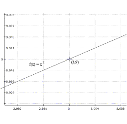
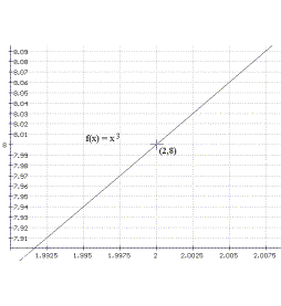
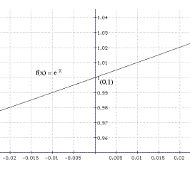
Here are some samples from sections of the graph of some
functions with the size of the viewing window. Based on
this information, estimate the slope of the tangent line
for each of these functions at the indicated point on the
graph.
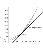

 e tangent to the
graph of $Y = X^2$ at the point (3,9). We
call a line that passes through two (or more) distinct
points on a curve a secant
line of the curve. As Figure 1 illustrates,
there are many secant lines to the graph of $Y = X^2$
that pass through the point (3,9). Each of these secant lines
is determined by the first coordinate of a point on the graph
of $Y = X^2$ other than (3,9). So using the
first coordinates 0, 1, 2, 4, 5, and 6 we have different
secant lines determined by the points (0,0), (1,1), (2,4),
(4,16), (5,25), and (6,36). A glance again at Figure 1
should help in understanding that the lines determined
by (2,4) and (4,16) are better
approximations for the tangent line than
the other lines in the figure.
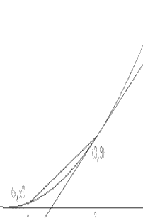
 denote $\bar
m (x)$. See Figure 5.
 Tangents constructed from
given points not on a curve. One of the traditional
problems for tangents and circles is to construct tangent
lines to a circle through a point given outside of the
circle. See Figure 7. The construction from the point P to
the circle with center O finds the midpoint M of the
segment $\bar{OP}$ and then constructs the circle with
radius $\bar{OM}$ and center $M$. The points where the two
circles meet are $T$ and $S$, and the lines $TM$ and $SM$
are both tangent to the circle.
 Use
the result of Example I.A.2 to find equations for any
lines that are tangent to the graph of $Y = X^2$
and pass through the point $(3,5)$.
