This page requires Internet Explorer
6+ MathPlayer
or Mozilla/Firefox/Netscape 7+.
Chapter 0.B Backgrounds for Calculus
(draft)
© 2002 M. Flashman.
August, 2006: This page now requires
Internet Explorer 6+MathPlayer
or Mozilla/Firefox/Netscape 7+.
2. Functions Introduction
and Review.
Preface: There
are many different kinds of numbers and ways to express,
compare, and relate them. Wherever we turn, whatever we
read, we find numbers used to describe situations while
the relations between numbers help us understand, plan,
and control these situations. The special kind of
relation between numbers that is called a function, first
recognized explicitly by Leibniz, evolved through the work
of the Swiss mathematician Leonhard Euler
(1707-1783) ( pronounced "Oiler") and the French
mathematician Joseph Lagrange (1763-1813) to become a
cornerstone for mathematics in the 20th century. Though
Newton, Leibniz and the other early developers of the
calculus did not have the current concept of a function to
assist them, we would handicap ourselves seriously if we
did not recognize and use the function concept today.
Most students in a precalculus course have had some
experience with functions in their previous studies. A
complete and detailed introduction and review of function
concepts and examples early in this course would delay our
reaching the object of our studies, the analysis of the
functional relations with calculus course. For
this reason, our review in this section will be limited to an
exploration of the basic nature of functions and ways
to think about functions that make sense for describing,
visualizing and analyzing them. Thus our attention is
directed primarily at functions and change. You will
find a catalog of definitions and fundamental properties of
functions in Appendix ***.
The Trip:
One simple and very useful context for understanding functions
is that of a car traveling on a road, what we might call "the
trip." Numbers that are interesting here are often found on
the dashboard of the car and by the roadside. They measure
such quantities as the amount of gas in the gas tank, the
distance traveled during this trip, the distance traveled by
the car since it was "new," the temperature of the engine, the mileage markers
on the side of the road, the speed limit markers, the
speedometer giving the car's speed, the tachometer indicating
the rate at which the engine is turning, and the clock.
For sure when we are considering any trip in a car
we are aware that time is changing whether the car is standing
still or moving very quickly. Thinking about the relations
between these quantities can help us gain some informal
understanding of functions and how they can be used to
understand the trip. For example, the distance the car has
traveled is related to the gas the car's engine has consumed.
The temperature of the engine is related to the rate at which
the engine is turning. All the measurements can be
thought of as related to time, since when we make a
measurement we do that at a particular time.
The concept of function can be
applied in many contexts beyond that of real numbers. For
the purpose of beginning our study of functions, we will
use the concept only for examining functions that relate
real numbers. These functions are usually described as
real valued functions of a real variable. Other
function concepts studied in mathematics treat relations
between three or more variable numerical quantities as well
as variables that are not numbers but geometric points and
vectors.
Static
Functions as Relations: The
mathematical concept of function connects quantities while
suggesting informally something stronger than just a relation
between the quantities. In one sense when we describe a
function relationship between variable quantities, we
are establishing a priority or an order to the information.
When two variables are related we often can identify one as
being an independent,
governing,
or controlling variable while describing the other as a
dependent, regulated, or controlled variable. These
descriptives indicate an important quality of a function,
namely that knowledge,
assignment, or specification of one variable's value will
determine the value of the other variable. In this
sense we can consider each of the variables in the trip
context as functions controlled by the time variable. It is
not that there is any necessary scientific or causal relation
between time and the position of the car (or any of the car
variables). The function language merely indicates that
knowing the time should allow us to determine the position of
the car.
A function connects the information about the variables by
pairing the data and assigning a priority to the pairs.
Knowing the first number of a pair uniquely determines the
pair, and thus the second number of the pair.
Dynamic
Functions - paired changes.
There is a second way to think of functions relating
variables. We consider the function as a mechanism
or interpreter that transforms one measurement or
number into a second number. [It helps to avoid
thinking of this process as being strictly causal in
physical situations, even though there is some strong
connection to causality with a priority to the order of
the relation.]
In the trip context we can think of the car dashboard as
a mechanism. Knowing the time by reading the clock
allows us to determine what the reading on the odometer
is. The distance our car has traveled is a function of
time. One can also connect the amount of gas in the
gas tank, measured by the gas gauge, to the distance the
car has traveled during a trip, thus the amount of gas
is a function of the distance traveled. |
The history of clocks and
watches and the measurement of time are a fascinating part
of the development of science and mathematics. Time
certainly plays an important role in our lives today, one
that we sometimes overlook too easily. We take for granted
our ability to measure time with precision to the
microsecond, but in 1773 the British government paid a
20,000 pound sterling prize to John Harrison for
developing a very accurate navigation chronometer with
which to calculate longitude. |
This mechanistic view of functions goes
particularly well with the use of calculators. You
enter a number on the display, push a single button and the
(resulting) number on the display is usually changed.
The terms "input" and "output" are
used here to describe the values of the controlling and the
controlled variables respectively. When thought of as a
machine, a function will process some numbers while being
unable to process others. For example, if the process returns
the multiplicative inverse (reciprocal) of a number, then the
process will work well on all numbers with the single
exception of 0. Or if the process returns the real number
square root of a given number, then the process will operate
on non negative real numbers but will fail to return a result
for negative real numbers. [Remember, the square root of a
negative number is not a real number, but an imaginary
number.]
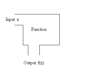
Figure illustrating a function machine.
|
|
We refer to the collection of numbers which
the function can process as the source or domain of the
function. Thus the function that returns the
reciprocal of a number has a source of the set of all non zero
real numbers, while the source for the real valued square root
function is the set of non negative real numbers. The source
of a function when not described explicitly is assumed to
contain all the inputs that work.
It is useful to describe the
source of a function so you can avoid errors that sometimes
arise from applying the function in meaningless situations.
The most common algebraic restrictions on the source of a
function arise from division by 0 and finding square roots
of negative numbers.
For example, the function which returns the
number `1/{1-x^2}` for an input of the number x can have
a source that includes all real numbers except 1 and -1.
As a second example, the
function that returns the number `sqrt{1-x^2}` for the input
number x can have a source that includes only
numbers in the interval [-1,1].
Notation for Describing Functions: As these
last examples demonstrate, it would be convenient to have a
notation that allows us to describe a function either from the
static view of a collection of ordered pairs or from the
dynamic view by designating what the function yields as output
for a specified, yet arbitrary, input. The notation and
vocabulary that has evolved (and is still evolving) must
distinguish at least three things: the first number of
the pair, called the argument or the input number, the
second number of the pair, called the result, value, or
the output number, and the designation or name for the
function.
|
Variable Relations: A traditional approach to this notation
considers 2 variable names, say x and y,
with x representing the first number for the
function and y representing the second number.
In this approach there is no name for the function,
only a statement that y is a function of x
and an equation describing an explicit relation
between the variables, such as y = 2x+3,
or an implicit relation such as `x =
y^2` and `y>=0`. This approach abuses the notation
since the letter y refers both to the number
and the function relation of that number to the
number x.
For example, when the function y is described
by the equation `y = 2x+3` we can determine the value of `y ` when `x = 6` by
substituting 6 for `x` in the
formula `2x+3` to find `y
= 2 (6)+3=15`.
The ordered pairs determined by this
function have the form `(x,y)` where `y=2x+3` or
`(x,2x+3)`. For `x =
6`, the information from the function
is that (6,15) is one of the pairs of the
function. The evaluation of y when
x=6 has a traditional notation of
`y| _{x=6}=``
2x+3| _{x=6}=2(6)+3=15`
|
Beware: A common error is
confuse the parentheses in this notation for the value
of a function for the parentheses used frequently
to collect terms in an expression to be treated as a
single number in some algebraic calculation like
multiplication.
By convention, when f is a function, the symbols
`f(t+5)` means the value of f for
the number described by `t+5`, it does not mean the
product of the number `f` by the number `(t+5)`.
|
Function
Values: A more contemporary
approach to the notation (based on the notation used by
Lagrange in his work at the end of the 18th century), with
which you are no doubt somewhat familiar, assigns to the
function a specific letter or symbol that suggests what
the function does or at least gives the function a
recognizable name.
For example, the function might be the square root function.
The square root function is assigned the shorthand name sqr,
or, as with less familiar functions, it might be named
temporarily for the purpose of discussion with the symbol f
or g. Once the name has been given, the relation
between input and output, argument and result, can be
described in a number of ways. A variable name is given,
or presumed, for the input, like x or t, and
then the output is described as the value of the function at
x or t, which is denoted most often as f(x)
or f(t).
Notice
that this last notation for the value of the function at x
has four symbols: f denotes the name of the function,
x denotes the name of the number to be input, the two
parentheses separate the name of the function from the name of
the variable.
A description of the function can then be
accomplished by giving a procedure for finding the value
of `f(x)`, such as `f(x)=2x+3`. Once `f` has been
described and thus defined for the purpose of discussion, the
notation allows us to denote the value of the function
that corresponds to the number 6 as `f(6)`. This number can be
computed using the defining equation: `f(6)=2(6)+3=15`.
Likewise the value of the function for the number `-4` is
denoted `f(-4)`, and can be computed to be
`f(-4)=2(-4)+3=-5`. For the expression `t+5`, which can
represent a number, the value of the function is denoted
`f(t+5)`, which can be simplified by using the definition of
`f` so that `f(t+5)=2(t+5)+3 = 2t+13`.
The
function
value
notation is sometimes combined with the two variable notation
in statements such as "suppose `y` is a function of `x`, with
`y=f(x)=2x+3`." Then evaluation can be expressed by the
equation: `y| _{x=6}=f(6)=2(6)+3=15`.
Transformation Notation: Another current approach to describing the
input/output information of a function is to give the name
of the function, then a name for an input variable followed
by an arrow and an expression describing the output that
results from the input. For example, `f : x ->
2x+3` or more generally `f : x -> y = f(x)`.
The arrow in the notation helps convey visually the dynamic
aspect of a function that transforms a number. This notation
helps underscore the active nature of those functions that
in some way do require a construction of the resulting
number values by some conceptual (and perhaps even
mechanical or electronic) process.
Multi-case
functions: In some contexts a function
cannot be described by a single simple algebraic formula
using well known conventional functions. This can be for
many reasons:
- There may be no algebraic formula that
captures that the relation;
- The function may arise from a non algebraic
context;
- The function may piece together some more
simple function.
To piece
together simple functions, the most common method is to
establish some tests on the source numbers. These tests
determine precisely what the appropriate method is for
determining the function's value.
Here is an example of a function F
defined by cases.
Case 1: if `x <= 0`, then `F(x) = 0`;
Case 2: if `0< x <4` then `F(x) = {x^2}/16`,
and
Case 3: if `4 <= x` then `F(x)=1`.
To use this definition of `F` we need to first check
under which case the argument for evaluation falls, then
follow the function's rule as appropriate.
So, to find `F(-3)` we see first that `-3` falls
under Case 1, so `F(-3) = 0`.
To find `F(3)` we check that `3` is under Case 2, so
`F(3) = {3^2}/16 = 9/16`.
Finally to find `F(5)` we use Case 3, so `F(5) = 1`.
The conventional notation for this function's definition
is expressed by a multi-lined equation: 
|
Functions and Tables: In some cases we do not know any formula
that precisely matches the pairings for a
function. This is in fact mot common when we
look at any function that arises from real world
phenomena. We may have a formula that
provides a good estimate or we have only some data
. Sometimes this data is measured and recorded at
selected numbers (or times). In this case the
information we have for the function may be
displayed in the form of a table.
For example if f
is the function recording the room temperature
we may know only that f(0) = 60, f(4)
= 55, f(8) = 65, f(12) = 68, f(16)
= 68, f(20) = 68, f(24) = 60. It
is convenient to put this data in a table. See Table 1.
Be careful not to assume too much about a
function that is represented only by a table of
values at selected numbers. For example,
although f(0)= 60 and f(4)=55,
you cannot assume that f(2) is between
60 and 55.
|
|
x
|
f(x)
|
|
0
|
60
|
|
4
|
55
|
|
8
|
65
|
|
12
|
68
|
|
16
|
68
|
|
20
|
68
|
|
24
|
60
|
Table 1
|
Non algebraic [Geometric]
Functions: If we think of the room temperature
function again, we can imagine a device recording the
temperature graphically with a sheet of paper moving
at a steady rate under a marking pen attached to a
temperature sensitive device that moves the pen depending on
the room temperature. This would give a rather different
record of the room's temperature as a function of time. Once
scales are established on the paper for the time and
temperature, we can give a better estimate of the
temperature at many different times by being able to read
the graph. This graphical presentation of a function gives
much more information than a table, but you should be
careful here as well not to infer too much from the graph,
especially since the mechanism, the recording instrument,
and the scales all can contribute to the imprecision of the
information.
Curves and coordinates in Cartesian geometry. Using
numbers
to study figures in geometry is not a very recent part of
mathematics. And using figures to study connections between
numbers is also not new to math. In your previous course work
you have studied the algebraic relations between coordinates
of points on lines, circles, and other curves and conversely
have graphed figures to illustrate the relation between
numbers involved in an equation. The key in these
correspondences has been the connection usually attributed to
Rene Descartes in analyzing curves with numbers through use of
common measurements and variables related by equations
determined by the geometry, called analytic (or Cartesian)
geometry.
Coordinate system analysis applied to planar
curves can lead to function relations that are commonly
encountered in science. Measuring devices record the changes
during some experiment as a curve. The variables connected
to the curve are associated with the experiment using
rectangular coordinates and then the curve is interpreted as
representing the relation between these variables. Without
any prior knowledge of the relation of the variables,
neither can be assumed to be controlling, but there is a
general convention to consider the horizontal, first
coordinate variable (X) as controlling with the vertical
and second coordinate (Y) as the controlled variable. But
for a curve to give a function relation between these
variable there needs to be more either understood implicitly
or made explicit.
In particular, when given a
value for X we need a way to determine a value for the Y
variable using the curve as the mechanism for that
determination. This is easy enough in many familiar cases.
For the given value of X, say a, find a point P on
the curve with that value as its first coordinate, i.e., P
has coordinates (a,b) for some number b. When
there is only one point P with first coordinate a on
the curve, then the value b is uniquely determined
by the curve, and b is the value of the Y variable
corresponding to a. In this case we say that the
curve has determined Y as an explicit function of X
and assume we are using the coordinate convention just
described.
The Slope of the Tangent to a Curve as a
Function: There are other functions we can associate
with curves in analytic geometry. For many curves we can
determine at each point on the curve a line that very close to
the point looks indistinguishable from the curve and yet close
to the point meets the curve only once. As mentioned in
section 0.A, these lines are sometimes referred to as touching
or tangent to the curve at the point, or tangent lines. To
repeat the example from 0.A, to find the tangent line to a
circle at a point P, you need only draw a radius from the
center of the circle to the point P and then construct the
line perpendicular to the radius at P, which by Euclidean
geometry must be the tangent line. So how does this give rise
to a function using numbers?
Consider the case when the
curve determines Y as an explicit function of X. For a given
value of X, say a, we again find a unique
point P on the curve with that value as its first
coordinate, i.e., P has coordinates (a,b) for a
unique number b. Now it sometimes turns out that we
can find a unique, non vertical tangent line to the curve
at P and determine the slope of this line, which we will
call m. Since the value of m is
uniquely determined using the curve from the value of X, m
is a function of X. The value of m is derived
geometrically from the original curve using the measurement
of the slope of the tangent line at the point P determined
by a.
Area of Geometric Figures as Functions: One
of the most frequently encountered problems in geometry is
that of finding a general method for determining the area
enclosed by a class of planar figures. You have learned
formulae for areas of squares, rectangles, triangles,
trapezoids, circles, and perhaps two or three other general
shapes. The measurement of these areas is usually based on
other measured features of the figures, such as lengths of
sides or relevant line segments and sometimes even the size of
angles.
The relationships between
area and these other variables of geometric figures can
often be described as functions. For example we can consider
rectangles that have a base of length 20 centimeters and
determine the area when the altitude has length l
centimeters. Not too hard.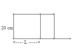
The area is 20 l square centimeters. Or in the same
setup, we can determine the length of the altitude when the
rectangle has area A square centimeters with almost
as little effort to be `A/20` centimeters. It requires a
little more thought to determine the length of the diagonal
of the rectangle with this setup based on the area A
to be `sqrt{A^2+1600}/20`.
Another familiar area relation is found in the
circle where the equation `A=pir^2` allows us to determine
either the area or the radius of a circle by knowing the other
measurement. A slightly more subtle area relation was described
in section 0.A. As the example there demonstrated there are many
ways to measure a region in the plane, like a triangle, and
passing a line across that region can give an area function
determined by the position of the line.
|
Implicit functions: Let's
consider the equation 3X + 4Y = 24 where X and Y
represent real numbers. There are many possible
choices for X and Y, some of which will make
the equation true (say X = 4 and Y = 3 ) and some of
which will not (say X = 1 and Y = 2). Given a value
for X there is one and only one value for Y
which will make the equation true. Thus if X = 1
then for the equation to be true we have 3 + 4Y = 24
, so 4Y = 21 and Y = 5.25. Since the equation
determines a unique value for Y from any choice of
X, we can say that the equation has determined Y
implicitly as a function of X.
A more subtle relation is presented by
the equation X 2 + Y 2 =
25. This equation can be satisfied by many
functions. For example `f(x)=sqrt{25-x^2}`,
`g(x)=-sqrt(25-x^2)`, or  . Here the
equation does not determine a single value of one
variable from the choice of another value but allows
many possible functions which will satisfy the
equation when the Y is determined by one of these
functions. In this case the functions are
described as being defined implicitly by the
equation. |
Comment: With only a
limited list of function values there is
no way to tell what the function might
have for its graph without assuming
some more restrictive qualities. For
example, suppose the graph of the function
is known to pass through two points with
coordinates (0,0) and (1,1).
You might think this is the function with
`f(x) = x`, but in fact it could be
`f(x)=x^2` or `f(x) = x^3` or
`f(x) = x^2 + x - x^3`.
In fact if we consider all functions with
f(0)= 0 and separately those
functions with f(1)=1, we are only
asking for those functions that satisfy
both conditions, which doesn't seem like a
large restriction when we think of all the
different ways we could connect the points
with coordinates (0,0) and (1,1) in a
Cartesian plane.
|
|
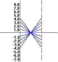
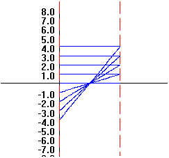
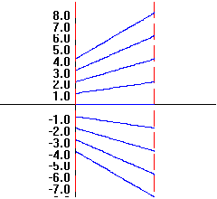
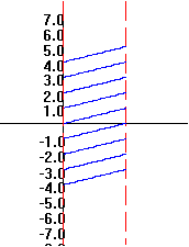
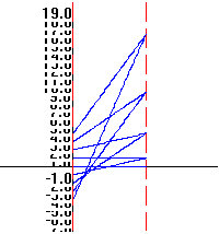
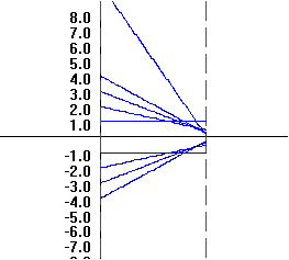
Visualizing Functions and
Transformation Figures: The key
idea in visualizing functions with mapping diagrams or
transformation figures is to have two parallel number
lines representing the source (domain) and the target
(range). The function can be thought of as a process
relating points (numbers) on these two lines.
A
point element on the source line is chosen which
corresponds to a number. The function is applied to that
number, and the resulting value is found represented on
the target line. An arrow drawn from the point on the
source line to the corresponding point on the target line
visualizes the relation between the corresponding numbers.
In one sense, the
transformation figure is a visualization of a
function table. The numbers in the two columns
of the table are represented by points on the
two lines in the figure. The function relation
that the table displays implicitly by having
corresponding numbers in the same row is
visualized in the figure by the arrow.
While the relative size of the numbers in the
target column of the table is not represented in
the display, the transformation figure uses the
number line order to represent this aspect of
the function's values.
Here is an illustration that
should help you see some of these features. You
can work on other examples after this one to
begin to see some of the power of this
visualization. [ To see a dynamic example of a
transformation figure for linear functions, follow
this link.]
Example:
Suppose f(x)=2x+ 3. Table 1
shows a selection of the values this function
relates, while this same information is visualized
in Figure 4. Notice that larger numbers in the
source column of the table correspond to larger
values in the target column. On the transformation
figure this feature can be seen by the fact that the
lines connecting the corresponding points on the
source and target lines do not cross. This is
evidence of a function with increasing values.
|
|
x
|
f(x)=2x+3
|
|
5
|
13
|
|
4
|
11
|
|
3
|
9
|
|
2
|
7
|
|
1
|
5
|
|
0
|
3
|
|
-1
|
1
|
|
-2
|
-1
|
|
-3
|
-3
|
|
-4
|
-5
|
|
-5
|
-7
|
Table 1
|
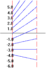 Figure 4
|
|
Graphs of Functions and Other
Relations: In your
previous work with functions and equations you have worked
extensively with the graphical visualization using Cartesian
coordinates for the plane to identify the function pairing
of numbers.
In the graph of a function f
we identify the pair of numbers a and f(a)
with the point in the plane with coordinates (a,f(a)).
We can plot marks at many of these points but when the
domain of the function is an interval or as is more common
all real numbers, we cannot hope to plot all the points.
Instead we try to give a sense of how the points are related
by drawing a curve that passes through some points that are
known to be on the graph of the function. In doing this we
are drawing figures much as students in elementary school
draw figures by connecting the dots in order, or as
economists graph the hour to hour price of some stock on the
stock market or as a chemist would visualize the minute by
minute temperature reading on a laboratory thermometer
during an experiment.
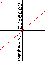
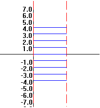
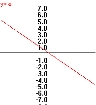
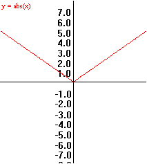
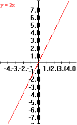
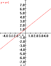
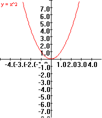
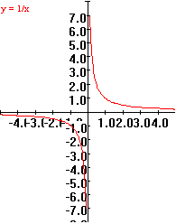
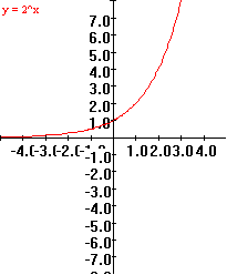
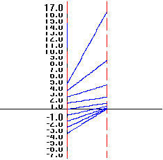
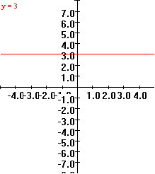
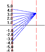
Here are some examples of
transformation figures and graphs. On the left are the
tables of values for the functions at selected points, while
on the right are the corresponding figures and graphs.
[Graphs and Figures made using Winplot.]
Example
0.B.2 f(x) = x
|
x
|
f(x)=x
|
|
2
|
2
|
|
1
|
1
|
|
0
|
0
|
|
-1
|
-1
|
|
-2
|
-2
|
|
 |
 |
Example
0.B.3 f(x) = -x
|
x
|
f(x)=-x
|
|
2
|
-2
|
|
1
|
-1
|
|
0
|
0
|
|
-1
|
1
|
|
-2
|
2
|
|
 |
 |
Example
0.B.4 f(x) = |x|
|
x
|
f(x)=|x|
|
|
2
|
2
|
|
1
|
1
|
|
0
|
0
|
|
-1
|
1
|
|
-2
|
2
|
|
 |
 |
Example
0.B.5 f(x) = 2x
|
x
|
f(x)=2x
|
|
2
|
4
|
|
1
|
2
|
|
0
|
0
|
|
-1
|
-2
|
|
-2
|
-4
|
|
|
|
Example
0.B.6 f(x) = x+1
|
x
|
f(x)=x+1
|
|
2
|
3
|
|
1
|
2
|
|
0
|
1
|
|
-1
|
0
|
|
-2
|
-1
|
|
 |
 |
Example
0.B.7 f(x) = x 2
|
x
|
f(x)=x
2
|
|
2
|
4
|
|
1
|
1
|
|
0
|
0
|
|
-1
|
1
|
|
-2
|
4
|
|
 |
 |
Example
0.B.8 f(x) = 1/x
|
x
|
f(x)=1/x
|
|
2
|
0.5
|
|
1
|
1
|
|
0
|
??
|
|
-1
|
-1
|
|
-2
|
-0.5
|
|
 |
 |
Example
0.B.9 f(x) = 2x
|
x
|
f(x)=2x
|
|
2
|
4
|
|
1
|
2
|
|
0
|
1
|
|
-1
|
0.5
|
|
-2
|
0.25
|
|
 |
 |
Example
0.B.10 f(x) = 3
|
x
|
f(x)=3
|
|
2
|
3
|
|
1
|
3
|
|
0
|
3
|
|
-1
|
3
|
|
-2
|
3
|
|
 |
 |
Example
0.B.11 f(x) =-2x + 1
|
x
|
f(x)=-2x+1
|
|
2
|
-3
|
|
1
|
-1
|
|
0
|
1
|
|
-1
|
3
|
|
-2
|
5
|
|
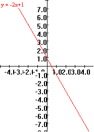 |
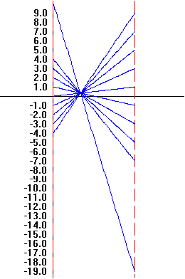 |
Using GeoGebra to do this:
You can move the point on the x axis in the mapping diagram see the function values vary with the
indicated value of x.
This point also moves the related point on the graph.
You can change the function definition for the
graph and the mapping diagram.
|
Martin Flashman,
26 June 2013, Created with GeoGebra
|
Review Exercises: The
exercises for this section cover material which you may recall
from previous course work in algebra and trigonometry. You may
not recall all of these topics or how to do the problems
precisely. You may want to refer to the texts or notes from
your previous courses in mathematics if you find these
difficult. The skills needed to solve these problems will be
important in the work ahead- so be careful to identify any
difficulties you have with these problems and try to remedy
any misunderstandings as you proceed.
1. For this problem let f be defined by `f (x)
= 5x^2 + 3`. a) Find the following. Simplify you answer
when possible. i)
`f(1)`
iii) `f(1+h)`
ii)
`f(h)`
iv)
`{f(1+h)
- f(1)\}/h`
b) Find any number(s) z where f(z) =
23. c) For which values of x is f(x)
< 23? Express your answer as an interval.
2. USING INTERVAL NOTATION, express the
largest set of real numbers that can serve as the domain of
each of the following functions:
a) `f(x) = (4 - x^2)/(x +
2)` b) `g(x)
= 1/(4-x^2)`
3. Suppose that F
is defined by  .
.
Sketch a transformation
figure and a complete graph of f.
Determine the domain and the range of f.
4. Solve for x:
a) 3 x-2 = 3
7-2x b) 4 3x
= 8 c) 1/3(x -
5) = 2 d) 1/30 - 1/x = 1/6
5. Boyle's law states that, for a certain gas P*V =
320, where P is pressure and V is volume.
(a) Draw a complete graph representing this
situation. Label your axes and write an equation for each
asymptote.
(b) If `8 <= V <= 40`, what
are the corresponding values of P?
6. Let f(x) = x
2 + 4x - 5. A. Find the axis of
symmetry and the vertex of f. B. Sketch a graph
of f labeling clearly the coordinates of the vertex
and the X- and Y- intercepts.
7. Old McDonald has a farm ,and on that farm she has
some sheep and a pasture with a 200 meter long stone
wall. She wants to enclose a rectangular section of the
pasture for a small sheep pen using the wall for one side and
140 meters of fencing she was given by her uncle Milo
for the other three sides.
A. Let x denote the length of the fence that will be
attached to the wall used as a side for the pen. Which
of the following equations express the area of the pen, A, as
a function of x?
a. A = x ( 70 - x)
b.
A
=
2
x ( 140 - x)
c. A = x ( 140 - x)
d.
A
= x ( 200 - (1/2)x)
d. A = 2 x ( 70 - x)
e.
A = 2 x ( 200 - x)
17. Write a short story
about cooking dinner. Discuss briefly those aspects of the
meal's preparation that might be related by functions.
18. Write a short story
about going shopping. Discuss briefly those aspects of the
shopping that might be related by functions.
19. Write a short
description of an ecological system. Discuss briefly those
aspects of the system that might be related by functions.
20. Write a short
description of the human body. Discuss briefly those aspects
of the body that might be related by functions.
21. Write a short story
about an athletic event or sports competition. Discuss briefly
those aspects of the story that might be related by functions.


 . Here the
equation does not determine a single value of one
variable from the choice of another value but allows
many possible functions which will satisfy the
equation when the Y is determined by one of these
functions. In this case the functions are
described as being defined implicitly by the
equation.


 .
.