Chapter VI.B Learning and Logarithms.

VI.B THE NATURAL LOGARITHM FUNCTION

Logarithmic functions are introduced in precalculus work with definitions related to exponential functions. For instance the logarithm with base 2 of the number N is defined by the statement that log₂(N) = x if and only if N = 2^x. [Or for a more specific example recall that log ₂(16) = 4 because 2⁴= 16]. This approach was made popular by Euler in his introductory mathematics textbook written in the 18th century. This was not the original definition of a logarithm given by Napier in the late 16th century based on rates and the convenience of the decimal notation for fractions. In this section we will study logarithmic functions starting with a model for learning. In this model we assume an individual learner (a person learning a language or a rat learning to master various mazes) has been involved in the process of learning for some time before we begin measuring. We assume that we can quantify and measure the amount that the learner has mastered at time t and we denote this quantity by L(t). [L(t) might be the number of words learned, the number of pages learned, or the number of mazes mastered. If we are looking for a measure that determines real numbers as results we could consider something like the actual distance travelled by the rat along the solution of a maze.]

For convenience we set our time units so that our measurements start when t = 1. Again for convenience we assume that L(1) = 0. This can be interpreted as the learner having a basic knowledge of the subject matter at the initial measurement time (t = 1). Alternatively at the initial measurement time we disregard what the learner has accomplished previously on the assigned task. Now to continue developing this model we will consider the situation where learning becomes more difficult as time proceeds (perhaps because of fatigue or progressively more difficult tasks to be mastered).

Models for Learning: We use a differential equation to model the increased difficulty in learning by assuming that the rate of learning is a decreasing function. A very simple model for this general context might have the rate of learning decreasing at a constant negative rate, such as L'(t) = -2t + 5, or perhaps when t >0 with a quadratic such as L'(t)= -2 t² + 12. You can pursue these examples further in the exercises at the end of this section. One thing about these two suggested models is that eventually L'(t) < 0, which we can interpret as saying that after a while the rate of learning is negative, or after a while the learner is forgetting.

One important yet simple model where the rate of learning is always positive, i.e., L'(t) >0 for all t, has the rate of learning inversely proportional to the time. I.e.,

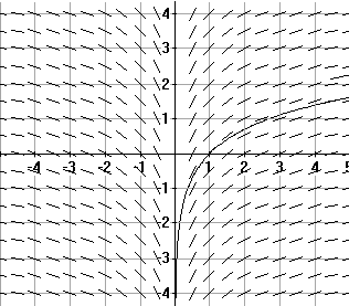
$L'(t) =\frac1t$, or, in Leibniz notation, $\frac{dL}{dt}= k\frac1t$ . This differential equation is the chief focus for this section. Notice first that with k>0, the derivative for all t>o is positive, so the learner is always learning more. By an appropriate choice of units we may assume that k = 1, so the differential equation of the model we will consider is $L'(t)=\frac1t$ with the boundary condition $L(1) = 0$.

Visualizing the solution: Following the work of Chapter IV, we draw the tangent fields for the equation $L'(t) = l/t$ to see the general shape of the particular solution as illustrated in Figure 1.

Figure 1

Tangent field and integral curve for $L'(t)=\frac1t, L(1)=0$.

We can analyze the function L using the 1st and 2nd derivatives to confirm the shape of the curve we find in the figure. $L'(t)= \frac1t >0$ for $t>0$, so $L$ is increasing for $t>0$, and $L''(t)= -\frac1{t^2} < 0$ for $t> 0$, so $L$ is concave down for $t> 0$.

A Learning Model Question: Let's consider the question, "How much is learned at time $t= 2$?" or, "What is the value of $L(2)$?" We can begin to estimate an answer by using Euler's method to approximate $L(2)$.

Table 2 Euler's method:
Estimate $L(2)$ from $L'(t)= \frac1t$ with $L(1)=0; n=4$.
t	L(t)	L'(t)=l/t	dL=.25/t
1.00	0.0000	1.0000	0.2500
1.25	0.2500	0.8000	0.2000
1.50	0.4500	0.6667	0.1667
1.75	0.6167	0.5714	0.1429
2.00	0.7595

In fact with $n= 4, dx =.25$, and $L(2)\approx .759524$. When $n=100, dx = .01$ and $L(2)\approx 0.69565343$. These are both overestimates because of the concavity of the solution. [See Table 2 or use this spreadsheet to make your own estimates.]

As we've seen in the Chapter IV discussion of the definite integral, Euler's method in the context where the derivative depends only on the controlling variable is another way to approximate the definite integral, $\int_{t=1}^{t=2} \frac1t dt $. In fact, this allows us to conclude that $L(2) = \int_1^2 \frac1t dt $.

Furthermore, if we let $G(x)=\int_{t=1}^{t=x} \frac1t dt$, $x>0$, then, by the derivative form of the Fundamental Theorem of Calculus (Theorem ***), $G'(t)=\frac1t$ for all $t> 0$ and by definition $G(1)= \int_{t=1}^{t=1} \frac1t dt=0$.

So $G(x)=\int_{t=1}^{t=x} \frac1t dt$ is the unique solution to the differential equation, $L'(x)=\frac1x$, satisfying the condition that $L(l)=0$. That is, for all $x> 0,

$$L(x) = G(x)=\int_{t=1}^{t=x} \frac1t dt.$$ [Can you interpet this integral as an area? See Figure 2.]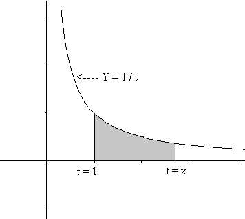

Figure 2

Note that if $0\lt x \lt 1$, then $G(x)=\int_{t=x}^{t=1} \frac1t dt >0$ so

$$L(x)=\int_{t=1}^{t=x} \frac1t dt=-\int_{t=x}^{t=1} \frac1t dt<0.$$ [Can you interpret this integral as an area? See Figure 3.]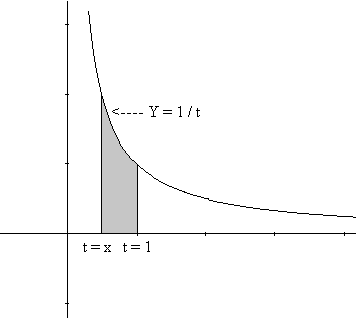

Figure 3

We can summarize these observations as follows:

For any x with $0 \lt x \lt 1$ , $L(x) < 0$, while when $x>1$, $L(x)>0$. [See the GeoGebra Figure below.]

Another Modeling Question: One more question for any learning model of is how much more will be learned if the learner spends more time at the effort. In particular, how much more will be learned if the learner spends twice as much time at the effort? In functional terms the question might be expressed: Can we relate the value $L(2x)$ to the value $L(x)$? The latter question has an unexpected yet simple answer in this model.

Let's think about this a little before we state and verify the solution using calculus.
If we consider everything the learner has learned up till time x as what has been learned in the initial time unit, then time x is just like time 1 originally. Now doubling the learning time spent can be considered what is learned at time $2x$ or at time $2$ originally. So the amount learned from time $x$ to time $2x$ should be the same as the amount learned from time $1$ to time $2$, i.e., since $L(1)=0$,

$$L(2x) - L(x) = L(2) - L(1) = L(2) .$$

Solution: For $x>0, L(2x)= L(2) + L(x)$.
Here's why. We can proceed with the same style of argument used in the previous section's discussion of the exponential function.

Consider the difference $F(x)= L(2x) - L(x), x>0$, representing the change in the amount learned from time $x$ to time $2x$ as a function of the variable $x$.
Then applying some simple calculus rules [including the Chain Rule] we see that $F '(x) = L'(2x)\cdot 2 - L'(x)$, so $F'(x>=\frac1{2x}\cdot 2 - \frac1x = 0$.
Hence the difference function $F(x)$ is a constant function [because $F'(x) = 0$].
But $F(1) = L(2)- L(1) = L(2) - 0 = L(2)$ [because we assumed $L(1)=0$].
So, $F(x) = L(2)$ for all $x>0$ , or $L(x) - L(t) = L(2)$ which justifies the claim

$$L(2x) = L(2) + L(x).$$

EOP.

Comment: This result is rather remarkable when interpreted in our model. If the learner doubles the time spent, the additional amount learned will always be the same, namely $L(2)$. Using the integration expression for the function $L$ and substitution we can find another justification for the result. The key to this justification is the fact that for any $x>0$,

$$\int_{t=x}^{t=2x} \frac1t dt=\int_{u=1}^{u=2} \frac1u du=L(2)$$ which can be seen using the substution $u =t/x$.

$u =t/x$
du = 1/x dt	t = x, u = l
1/t dt = 1/ux xdu = 1/u du	t = 2x, u= 2

Thus $$L(2x)=\int_{t=1}^{t=2x} \frac1t dt$$ $$=\int_{t=1}^{t=x} \frac1t dt + \int_{t=x}^{t=2x} \frac1t dt$$ $$=\int_{t=1}^{t=x} \frac1t dt + \int_{u=1}^{u=2} \frac1u du$$ $$=L(x)+L(2)$$ In fact, as the next theorem shows, there was nothing special here about the number $2$.

Theorem VI.B.1: For any $a>0$ and $x>0, L(ax) = L(a) + L(x)$

Proof: We follow the same organization as in the previous solution discussion.

Let $F(x)= L(ax) - L(x), a>0, x>0$,
Then applying calculus rules we see that $F '(x) = L'(ax)\cdot a - L'(x)$, so $F'(x)=\frac1{ax}\cdot a - \frac1x = 0$.
Hence the difference function $F(x)$ is a constant function [because $F'(x) = 0$].
Again, $F(1) = L(a)- L(1) = L(a) - 0 = L(a)$.
So, $F(x) = L(a)$ for all $x>0$ , or $L(ax) - L(t) = L(a)$ which justifies the theorem

$$L(ax) = L(a) + L(x).$$

EOP.

Comment. You should draw some figures that visualize the geometric interpretation of this theorem for several situations depending on whether or not $a> 1$ and $x> 1$. You can also give an alternative justification for this result using the definite integral characterization of the function L and substitution.

More Properties of L: We can restate the last result a little differently by letting $ax = s>0$ so that $a= s/x$. Then $L(s) = L(s/x) + L(x)$. So we've shown

Corollary VI.B.2: $L(s/x) = L(s) - L(x)$ for any $s, x > 0$.

Note further that when $s = 1$ we've shown that $L(1/x)= L(1)- L(x)= 0 - L(x)$. So we have

Corollary VI.B.3: $L(1/x) = -L(x)$ for $x> 0$.

Another Modeling Question: While we're noticing some of these algebraic properties of the function $L$, let's consider what the effect is of allowing a learner to work for a time that is a power of the original time $t$.

For example, what is the relation of $L(t^5)$ to $L(t)$?

Solution: This question is not hard to answer because of our previous results:

$L(t^5) = L(t\cdot t^4) = L(t) + L(t^4)$

$= L(t) + L(t \cdot t^3) = L(t) + L(t) + L(t^3)$
$= ... = L(t) + L(t) + L(t) + L(t) + L(t) = 5L(t)$.

You might expect the generalization of this solution to integer powers of $t$, but we can now generalize this example to all rational powers.

Theorem VI.B.4: If $r$ is any rational number, then for any $t> 0,\ L(t^r) =rL(t)$.

Proof: This time we consider the function F(t) = L(t ^r) - rL(t) for t > 0. F(t) measures the difference between the two quantites we hope to show to be equal.

Then F '(t) = L'(t^r) r t ^r-1 - r L'(t)

[again, we used the Chain Rule] so F '(t) = 1/(t^r ) rt^r-1 - r l/t = r/t - r/t = 0.

Thus F(t) is a constant function. But F(l) = L(l ^r) - rL(l) = 0 - 0 = 0 so F(t) = 0 for all t > 0.
Thus L(t ^r) - rL(t) = 0 or L(t ^r) = rL(t) .

EOP

Comments: 1. Again this last result can be obtained from an appropriate substitution in the definite integral that characterizes L.

2. These last few results are certainly consistent with what we might suspect for a logarithmic function. We'll discuss this again later in this section.

The Bounded Learning Question: Let's return to our learning model to ask another rather interesting question. If the learner has unlimited time, is there any limit to the amount of learning that can be mastered? Suppose for example we want to be sure that at some time t, L(t) >100. How long should we be prepared to wait? That is, what value should we use for t so that L(t) > 100?

Solution: Here our last result and our earlier integral characterization of L(2) will help.

Figure 4

To begin, notice we can estimate

quickly, though less precisely than we did initially in this section. Using Figure 4 to illustrate the approximation geometrically we have 1/t > 1/2 for t between 1 and 2, so (from the monotonicity property of the definite integral) we have

> 1/2. Using the previous algebraic result, L(2^N) = N L(2), we have L(2^N) > N/2.
We can use t = 2 ^N to give a number t where L(t) > N/2. To find an appropriate t where L(t)> 100, we need only find N where N/2 > 100. In particular we can use N = 201, which shows we can solve the problem by using t = 2²⁰¹since L(2²⁰¹)= 201 L(2) > 201/2 > 100

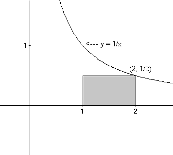
Well, 2²⁰¹ is a very large value for t, but it will work. And similarly we can show that if B is any number, there is some value for t where L(t) > B. In other words, since L is an increasing function, we have shown that .

You probably have noticed by this time that the solution to the differential equation L'(t) =1/t with L( 1) = 0 has practically all of the properties found in logarithmic functions. Because the function L satisfies all the properties of other logarithmic functions, the function L is usually called the "natural logarithm function" and conventionally, when t > 0, L(t) is denoted ln(t). [The letters ln stands for the Latin words, logarithmus naturalis.
Thus, using this conventional notation ln for the function L, we have that for all x > 0,

We continue to study this function more extensively in the next few sections, but for now we close our discussion with an example that applies basic properties of the natural logarithm to find the derivatives of some complicated functions.

Example VI.B.1. Find the derivatives of the following functions.
a) $y = f(x) = \ln(x^2+ 1)$;
b) $y= f(x) =\ln(\sin(x))$ for $0< x <\pi$
c) $y=f(x) = \ln(\frac{x^2+ 1}{\sin(x)})$ for $0< x <\pi$.

Solution: The first two of these are merely applications of the chain rule.
In a) let u = x²+ 1 so y = ln(u) and f '(x)=dy/dx = dy/du du/dx = 1/u 2x =2x/(x²+ 1).

In b) let u = sin(x) so that y = ln(u) and
f '(x) = dy/dx = dy/du du/dx = 1/u cos(x) = cos(x)/sin(x) = cot(x).

For c) we use the division property of the logarithm [Cor. VI.b.2] to see that

f(x) = ln(x²+ 1) - ln(sin(x)). Using the linearity of the derivative together with the results of parts a) and b) we find f '(x) = 2x/(x²+ 1) - cot(x).

Historical Note on Natural Logarithms and Areas. The area of the region of the plane enclosed by the graph of Y= l/X, the X-axis, the lines X=1 and X=t, was noticed to have logarithmic properties by the Belgian mathematicians Gregory of St. Vincent and Alfonso Antonio de Sarasa in the middle of the 17th century. This was just before the work on the calculus by Newton and Leibniz but more than 20 years after the initial development of logarithms by John Napier and Henry Briggs. For many years logarithms based on Y= l/X were called hyperbolic logarithms since the graph of Y=1/X is an hyperbola.

Logarithmic differentiation: The next example illustrates a technique referred to as logarithmic differentiation. It is very useful for finding derivatives of complicated functions. It will be used later in this chapter to explore more completely the derivatives of functions with complicated exponents.
Example VI.B.2: Find the derivative of y = (x² + 1) (x⁴ + 3)

Solution: We first consider ln(y) = ln( (x²+ 1) (x⁴+ 3)). Using the addition property of ln we have

ln(y) = ln(x²+ 1) + ln(x⁴+ 3). Although y has a derivative that can be determined from the product rule, we can use implicit differentiation on this last equation to find that derivative with only the sum and chain rules. $$\frac{d}{dx} ( \ln(y)) = \frac{d}{dx} (\ln(x^2+ 1) + \ln(x^4 + 3)).$$
This gives us $$\frac 1y \frac{dy}{dx} = \frac{2x}{x^2 +1} + \frac{4x^3}{x^4 + 3}.$$ [Don't forget the chain rule!] Now we solve for the derivative to find $$\frac{dy}{dx} = y[\frac{2x}{x^2 +1} + \frac{4x^3}{x^4 + 3}].$$ When we substitute the original expression for $y$ into this last equation we find $$\frac{dy}{dx} = 2x(x^4 +3) + 4x^3(x^2 + 1),$$ the result we could have obtained directly from the product rule.

To summarize, here is the process we used for logarithmic differentiation:

First we considered $\ln(y)$.

Then we used a properties of $\ln$ to simplify the operation involved in describing $\ln(y)$. [Multiplication became addition.]

After simplifying, we differentiated the resulting equation implicitly and solved for the derivative.

Finally we replaced $y$ with its initial expression to obtain the derivative of $y$ in terms of $x$.

Exercises VI.B.

Find the derivatives of the functions as indicated. [Don't forget the chain rule!]

f(x) = ln(5x), x > 0. Find f '(1), f '(2)and f '(t).
f(x) = ln ( -x), x < 0. Find f '(- 1) , f '(-2) and f '(t) for t < 0.
f(x) = ln (x ²) , x ¹ 0. Find f '(l) , f '(-l) and f ' (t).
f(x) = ln (sec (x)), -p /2< x < p / 2. Find f '(0), f '(p/4) and f ' (t).
f(x) = ln(exp (x)). Find f '(0) , f '(l) and f '(t).

Find the derivatives of the functions as indicated. [Don't forget the chain rule!]

y = ln(3x) ,x >0. Find dy/dx when x = 1 and 2.
y = x ln(x), x>0. Find dy/dx when x = 1 and 2.
y = ln(x) sin(x) , x > 0. Find dy/dx.
y = ln(x ^1/2(x+l)), x>0. Find dy/dx when x = l.
y = ln(x ^1/2/(x+l)), x>0. Find dy/dx when x = 1.

Find the derivatives of the functions as indicated. [Don't forget the chain rule!]

Find D_t (sin(ln(t)) , t > 0.
Find D_t ln(t²- 1)), -l <t < 1.
Find D_t ( ln(t sin(t) )), 0 < t <p .
Find D_t (ln( t )/ t²), t> 0.
Find D_t (ln(sec(t) + tan(t) ), -p / 2 < t <p / 2

Sketch a graph of y = ln(x²+ 1) showing all extrema and points of inflection. Explain your work using first and second derivative analysis.
Sketch a graph of y = x ln(x), x > 0, showing all extrema and points of inflection. Explain your work using first and second derivative analysis.
Sketch a graph of y = x²ln(x), x >0, showing all extrema and points of inflection. Explain your work using first and second derivative analysis.
Sketch a graph of y = sin(x) ln( x ) for x in (0, 4p ], showing all extrema and points of inflection. Explain your work using first and second derivative analysis.
Show that y = k ln(x) + A is a solution to the differential equation y'= k/x with y(l)=A.
(Project) Other models for learning uses a simpler or decreasing functions that have easier differential equations to solve. Suppose L'(t)= t + 5 and L(l) = 0. Explore the same questions for this model that were examined in this section, namely, a) find L(2), b) try to relate L(t) with L(2t) and c) what can you say about the value of L when t is large? Generalize this example to all linear expressions for L'(t) with negative slope.
(Project continued.) As in problem 9), explore the model for learning that assumes L'(t) = 1/t²for t >0 and L(l)=0.
(Project) Suppose A'(t) = 1/(t²+ 1) and A(l) = 0. Compare this model to the model in the previous problem. Explain why for any t> 1, the solution for this differential equation A has A(t) <L(t) where L solves the differential equation of 10). What can you say about the value of A (t) when t is large?
Suppose f(x)= k/x is the probability density function for a random variable X on the interval [1,2]. Show that k = 1/ ln(2).
Find the following indefinite integrals:

Find the following definite integrals. You may express your answer using natural logarithms.

Using rectangles and the area interpretation of the definite integral explain why there is a unique number c between 2.5 and 3 where ln(c)= 1. Can you find a better estimate for c? Explain.