Preface: Throughout this introduction to calculus we have found that estimates could be improved by some process determined by a natural number n. In our estimates for solving equations this number n denoted the number of steps we would follow in using either the bisection method or Newton's method. Later n was the number of steps we used in Euler's method to estimate the value of the solution to a differential equation with given initial (or boundary) condition. Later still we found n controlling the size of intervals and the quality of estimates for the value of a definite integral with the trapezoidal rule and Simpson's rule. The number n also was used in estimating the values of many measurable quantities in applications, such as area and volume, allowing us to connect real situations to the mathematical concepts of derivative and integral. Finally, in the last chapter we found n indicating the degree of the MacLaurin and Taylor polynomials and their remainder terms which gave estimates for values for functions, integrals and solutions to differential equations.
The mathematics of real number sequences concerns the study a collection of real numbers determined in an order by a counter or index number, often denoted by n. The mathematical issues entail the description of these sequences and their properties.
One crucial question considers whether there is a tendency in the sequence for its members associated with larger natural numbers to approach a particular value called the limit of the sequence. There are actually two important and related questions:
(1) Is there a limit for a particular sequence?
For example, we are fortunate sometimes when we can use the Fundamental Theorem of Calculus to determine the precise value of the limit of numbers arising from Simpson's Rule for estimating a definite integral. Or in other situations we can use the Taylor Theorem to recognize that 1 + 1 + 1/2 + 1/6 + 1/4! + + 1/n! is approximately e. And we shouldn't forget that the sequences that arise from Newton's method for estimating solutions to equations (square roots, etc) frequently converge to numbers that are well described but known primarily by their estimates.
| {a n : n = 0,1,2, } | {b k}k = 0,1,2, | {c k}k = 1,2,3, |
| {x n}n = 0,1,2, | {y n} n = 0,1,2, | {s n} n = 0,1,2, |
A typical defining statement for a sequence is a n = f (n) where f is some function defined at least on the natural numbers For example an = n2, bn = 1/(n+1); xk = 1/k!; and s n = Sk=0k=n 1/k!.
An even more general example would allow the sequence to have a real variable in its definition, such as
Visualizing sequences: There are many ways to think about real number sequences and each way leads to a visualization of the sequence that can assist in making the sequence and its properties more apparent.
First, a real number sequence is a set of real numbers together with
an order for these numbers. With this in mind we can display
the sequence as a collection of points on a real number line. The
order of the points can be seen by labeling the points with the subscripts
that indicate there relative
order, such as a 1, a 2, a 3,
.
Example. X.I.A
A visualization of the sequence {1, 1/2, 1/3, 1/4, 1/5, 1/6, 1/7, 1/8,
1/9, 1/10, ..., 1/k ,...}

Another way to indicate the order is to draw an arrow from one point to the next on the line, so we see a succession of arrows above the number line each showing which number is next in the sequence.
A second and important way to treat a sequence is as a function
from its index set , usually the natural  numbers,
to the real numbers. [The expression of the definition of a sequence
by an equation like an = f (n) uses precisely this approach.]
Now we can visualize a sequence just as we visualize other functions, either
with a transformation figure from the source real number line to a target
real number line or with the graph of the function in the cartesian plane
of ordered pairs of real numbers.
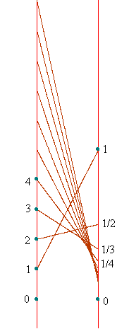
Example. X.I.A (continued). Let an = 1/n for n
= 1,2,3,... .
In the transformation figure the index values, n, will be located on
the source line while the actual values of the sequence, an,
will be corresponding points on the target line. An arrow is drawn from
the index point in the source to the corresponding value point of the sequence
on the target.
In fact the target line will look essentially like our first visualization without arrows to indicate the order. The order in the transformation figure is indicated by the usual order of the indices on the source line.
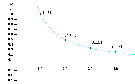
In the graph of a sequence we see a collection of points in the plane
with ordered pairs of real numbers for coordinates. The first coordinate
is the index of the number in the sequence, n, while the second coordinate
is the actual value of the sequence, an. The order in the graph
is seen as the fact that values with larger indices are represented by
points further to the right on the graph.
Convergence. The values of a real number sequence can be interpreted as numbers that occur in some order, as the image values in a transformation figure with the indices increasing, or as points on the graph of the sequence.
One issue that is very important in the study of sequences is whether
the values of the sequence
{an }n=0,1,2,
approach a limiting number,
L, when n is very large.
If this is the case we write that an ®
L as n ®¥ or lim n ®
¥ {an} = L and we say,"The sequence
an
converges to L as n goes to infinity."
Examples. Let a n = n2 ,b n
=1/(n+1), c n = 4n2 /(7 n2 - 5n
- 2), and S n = cos(1/(1 + n2 )).
Discussion: These sequences might also be described directly
as { n2 }n = 0,1,2,
; { 1/{n+1} }n
= 0,1,2,
; 4 n2 /{7 n2
- 5 n - 2} }n = 0,1,2,
; and {cos(1/(1 + n2)) n
= 0,1,2,
. Table X.A.1 shows some of the
initial values for the sequences while the figures below show in part the
tranformation figures and graphs for initial values of the latter three
sequences.
Without being rigorous at this stage, it should make sense that there
are limits for all but the first of these sequences. In particular
lim n ® ¥1/(n+1) =
0 ; lim n ® ¥ 4n2
/(7 n2-5n-2) = 4/7; and lim n ®
¥cos(1/(1 + n2 )) = 1.
Examples from Euler's method, Riemann sum integral approximations.
Example. A sequence that converges to e. Recall that in considering the differential equation y'=y with y(0)=1 we estimated the value of y(1) using Euler's method in n steps to be (1+1/n) n. With n larger we obtain better estimates for y(1)=e. Thus we can conclude that as n®¥ , (1+1/n) n ® e.
Example. A sequence that converges to ln(2). In considering the differential equation y'=1/x with y(1)=0, using Euler's method in n steps, we estimated y(2) » 1/n [1 + n/(n+1) + n/(n+2) + . + n/(2n-1)] = 1/n + 1/(n+1) + + 1/(2n-1) = S n. Thus as n®¥ , S n ® y(2) = ln(2). Notice that this sequence is also the sequence of left hand endpoint Riemann sum estimates of the definite integral ò121/x dx.
Example. A sequence that converges to 1/2. For a simpler example we can consider S n = 1/n [ 1/n + 2/n + . + (n-1)/n], the left hand Riemann sum estimate for the definite integral ò01x dx = 1/2 . Thus as n® ¥, S n® 1/2.
Examples from Taylor approximations.
Example. Another sequence that converges to e. Recall that in considering the differential equation y' = y with y(0)=1 we estimated the value of y(1) using Taylor (Maclaurin) polynomials of degree n evaluated at x=1. If we let Sn = Pn (1) = 1 + 1 + 1/2 + 1/3! + 1/4! + ... + 1/n!, then with n larger we obtain better estimates for y(1)=e. [In fact we actually have a measure of the difference between e and Sn given by Rn = e - Sn as in the work on Taylor Theory in chapter IX.] Thus we can conclude that as n®¥, Sn ® e. Furthermore, the same theory explains why for each x, the sequence Sn = Pn (x) = 1 + x + x2/2 + x3/3! + x4/4! + ... + xn/n! converges to ex as n®¥.
Example. A sequence that converges to ln(1.1). Recall that in considering the differential equation y' = 1/x with y(1)=0 we estimated the value of y(1.1) using Taylor polynomials of degree n about x=1 evaluated at x=1.1. If we let
Recursive (inductive) Definitions for Sequences
In the examples we have considered so far, each term of the sequence was defined without reference to previous terms. For example, consider the following sequences:
It is not difficult to see that each term in these sequences is related
to the next term.
Thus an+1= (1/2) an with
a0 =1; bn+1= 2 bn with
b0 =1; and cn+1= (n +1)
cn
with c0=1.
This connection between the terms in a sequence can be used to determine
the value of any particular term by moving step be step from the initial
value to the desired value using the relation at each step. So for example,
c1= (1) c0 = 1; c2=
(2) cn1 = (2) 1=2; c3= (3) c2
= (3) 2 = 6;...
Defining a sequence by giving an initial value and a relation between one term and the next term is described as "a recursive sequence" or "an inductive sequence."
Another example of a recursive sequence, called the Fibonacci sequence,
f
n
is given by two initial values, f0= 0,
f1 = 1 and the relation fn+2=
fn + fn+1. The first
12 terms of this sequence are 0,1,1,2,3,5,8,13,21,34,55,89.
Another example of a recursive sequence we can consider Newton's
method used to estimate the root of a function f. x0
is the inital estimate for the root for f (x) = 0.
The recursive formula that determines the next estimate is given by xn+1=
xn-
f(xn)/f '(xn ).
Using f(x)= x2 -2, and x0=
1, we have xn+1=
xn-
(xn2 -2) /(2xn ) = (xn2
+ 2) /(2xn ) and xn
approaches the square root of 2 as n ®¥
.
Exercises X.A.
For each of the following sequences, (a) list the first five values,(b) draw a transformation figure for the first five values, (c) draw a graph for the first five values, and (d) find the limit as n®¥ when possible.
1. (5n2 + 3n -2)/(2n2 + 3n -1) {n = 0,1,2 ...}.
2.sin( (3n -2)/(2n2 + 3n -1)){n = 0,1,2 ...}.
3. (4n + 2)/(3n2 + 2n -1) {n = 0,1,2 ...}.
4. (n3 + 1)/(3n2 + 2n){n = 0,1,2 ...}.
5. (-1)n{n = 0,1,2 ...}.
6. (-1)n/(n2 + 1) {n = 0,1,2 ...}.
7. (2/3)n {n = 0,1,2 ...}.
8. (-2/3)n{n = 0,1,2 ...}.
9. e1/(n+1) {n = 0,1,2 ...}.
10. arctan(1 - 1/(n+1)){n = 0,1,2 ...}.