MAA Minicourse #7 ¤
January 7 and 9, 2015 Making Sense of Calculus with Mapping Diagrams
Martin Flashman
Professor of Mathematics
Humboldt State University
Link for these notes: http://flashman.neocities.org/Presentations/MD.JMM.Mini.1_7_16.html
Abstract:
In this mini-course participants will learn how to use mapping diagrams
(MD) to visualize functions for many calculus concepts. For a given
function, f, a mapping diagram is basically a visualization of a
function table that can be made dynamic with current technology. The MD
represents x and f(x) from the table as points on parallel
axes and arrows between the points indicate the function relation. The
course will start with an overview of MD’s and then connect MD's to key
calculus definitions and theory including: linearity, limits,
derivatives, integrals, and series. Participants will learn how to use
MD’s to visualize concepts, results and proofs not easily realized with
graphs for both single and multi-variable calculus. Participants are
encouraged to bring a laptop with wireless capability.
What is a mapping diagram?
Introduction and simple examples from the past: Napiers Logarithm
Linear Functions.
Understanding functions using tables. mapping diagrams and graphs.
Functions: Tables, Mapping Diagrams, and Graphs
2. Linear Functions. ¤
Linear functions are the key to understanding calculus.
Linear functions are traditionally expressed by an equation like : $f(x)= mx + b$.
Mapping diagrams for linear functions have one simple unifying feature- the focus point, determined by the numbers $m$ and $b$, denoted here by $[m,b]$.
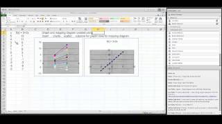
Mapping Diagrams and Graphs of Linear Functions
Visualizing linear functions using mapping diagrams and graphs.
Notice how points on the graph pair with arrows and points on the mapping diagram.
3.Limits and The Derivative ¤ Mapping Diagrams Meet Limits and The Derivative
3.1 Limits with Mapping Diagrams and Graphs of Functions
The traditional issue for limits of a function $f$ is whether $$ \lim_{x \rightarrow a}f(x) = L$$.
The definition is visualized in the following example.
Mapping diagrams and graphs visualize how the definition of a limit works for real functions.
Notice how points on the graph pair with the points and arrows on the mapping diagram.
3.2 The derivative of $f$ at $a$ is a number, denoted $f'(a)$, defined as a limit of ratios (
average rates or slopes of lines). i.e., $$f'(a) = \lim_{x \rightarrow a} \frac {f(x)-f(a)}{x-a}.$$
The derivative can also be understood as the
magnification factor of the best linear approximating function.¤
The derivative can be visualized using focus points and derivative "vectors" on a mapping diagram.
3.3 Mapping Diagrams for Composite (Linear) Functions ¤
This is the fundamental concept for the chain rule.
Visualizing the composition of linear functions using mapping diagrams and graphs.
Notice how points on the graph are paired with the points and arrows on the mapping diagram.
3.4. Newton's method. An early application of the first derivative, Newton's method for estimating roots of functions is visualized with
mapping diagrams.
The traditional analysis of the first derivative is visualized with
mapping diagrams. Extremes and critical numbers and values connected.
Time permitting- the Intermediate and Mean Value Theorems are
visualized.
3.5.1 First [and Second] Derivative Analysis.
Graphs of functions and mapping diagrams visualize first and second derivative analysis.
Notice how the points on the graph is paired with the points on the mapping diagram.
4Differentials, Differential Equations, and Euler's Method ¤
The major connection between the derivative and the differential is
visualized by a mapping diagram.
4.1 Mapping Diagrams for the Differential
Mapping Diagram for the Differential
Notice how the points on the graph are paired with the points and arrows on the mapping diagram.
4.2 Differential Equations, Euler, Mapping Diagrams ¤ Iterating the differential gives a
numerical tool (Euler's Method) for estimating the solution to an
initial value problem for a differential equation.
$P(x,y)= \frac {dy}{dx}, f(a)=c$
Estimate $f(b)$ given $y'= P(x,y)$ and $f(a)=c$ in N steps. $ \Delta x = \frac{b-a}N; f(b) \approx f(a) + \sum_{k=0}^{k=n-1} P(x_k,y_k)\Delta x $
5 Integration and the Fundamental Theorem
Connecting Euler's method to sums leads to a visualization of the
definite integral as measuring a net change in position in a mapping
diagram and an area of the graph of the velocity. Definition: The definite integral of $P$ over the interval $[a,b]$, denoted $\int_a^b P(x)dx$, is defined as the number $I$, where as $N \rightarrow \infty$, $\Delta x
\to 0$, $$\sum_{k=0}^{k=N-1} P(x_k)\Delta x \rightarrow I \equiv
\int_a^b P(x)dx, \ provided\ the \ limit, I , \ exists.$$ Theorem:
Suppose $P(x)$ is a continuous function on $[a,b]$, then $\int_a^b P(x)dx $ exists.
The Additive Property for Integral Theorem:Suppose $y = P(x)$ is a continuous function on $[a,c]$ and $ a<b<c$ then
5.1 Euler's Method visualized with mapping diagram and graph, showing
the connection between the mapping diagram and the area of a region in
the plane bounded by the graph of
$y = P(x) = f'(x)$, the X axis, X=a and X
= b.
Move the sliders to change $a,b$, and $N$. You can also change the
function $P(x) = f'(x)$ by entering a new function in the box.
5.2 SC STUFF
[The Additive Property.] $\int_a^b P(x) dx = \int_a^c P(x) dx + \int_c^b P(x) dx$ for any $a, b,$ and $c$.
Geometry Interpretation: If $P(x) > 0$ and $a < c < b$ , then
the area of the regions above the $X$-axis and below the graph of
$Y=P(X)$ between the lines $X=a$ and $X=b$, $\int_a^b P(x)
dx$ , is the sum of the areas of the regions enclosed by the $X$-axis,
the graph of $Y=P(X), X=a$ and $X=c$, $\int_a^c P(x) dx$ , and by the
$X$-axis, the graph of $Y=P(X), X=c$ and $X=b$, $\int_c^b P(x)
dx$ .
See Figure V.B.1.
Motion Interpretation: Assume $a < c < b$. The net change in
position of an object moving with velocity $P$ between time $a$ and
time $b$, $\int_a^b P(x) dx$, is the sum of the net changes in position
between time $a$ and time $c$, $\int_a^c P(x) dx$, and between time $c$
and time $b$, $\int_c^b P(x) dx$. See Figure V.B.1.
Figure V.B.1.
These properties allow some determination of definite integrals based on
knowledge of the components that make up the integrand. Although the
calculus is not as easy as that of the derivative here are some examples
of how the properties just discussed can be used for an elementary
calculus for the definite integral.
End SC STUFF
The additive property of the definite integral visualized with mapping diagram and graph, showing
the connection between the mapping diagrams and the areas of regions in
the plane bounded by the graph of
$y = P(x) = f'(x)$, the X axis, X=a, X
= b, and X =c.
Move the sliders to change $a,b,c$, and $N$. You can also change the
function $P(x) $ by entering a new function in the box.
Mean Value Theorem for Integrals:
If $p$ is a continuous function on $[a,b]$ then there is an number $c_* $ between $a $ and $b $ where
$$\int _a^b P(x) dx = P(c_*)*(b-a).$$
The Fundamental
Theorem of Calculus.Suppose $y = P(x) = f'(x)$ is a continuous function, then
$$\int_a^b P(x)dx + f(a) = f(b)$$
or
$$\int_a^b P(x)dx = f(b) - f(a)$$
where $f'(x) = P(x)$.
5.3 Euler's Method visualized with mapping diagram and graph, showing
the connection for the Fundamental Theorem of Calculus between the mapping diagram and
$$\int_a^b P(x)dx = f(b) - f(a)$$
where $f'(x) = P(x)$.
Move the sliders to change $a,b$, and $N$. You can also change the
function $P(x) = f'(x)$ by entering a new function in the box.
7.1 GeoGebra Applet for visualizing sequences with Mapping Diagrams and Graphs for a sequence defined by $a_n = f(n)$
8.1 GeoGebra Applet for constructing MacLaurin Polynomials and Remainders $P_n(x,f(x))$ and $R_n(x,f(x))$


 AMATYC Webinar Martin Flashman - Using Mapping Diagrams to Understand Functions (YouTube)
 AMATYC Webinar M Flashman Using Mapping Diagrams to Understand Trig Functions (YouTube)
 Martin Flashman ...Solving Linear Equations Visualized with Mapping Diagrams (YouTube)
 Martin Flashman ...Partial Derivatives: An Introduction Using Mapping Diagrams (You Tube)