5.4.1
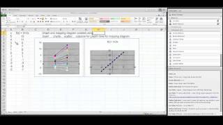
Euler's Method visualized with mapping diagram and graph, showing
the connection for the Fundamental Theorem of Calculus between the mapping diagram and estimating
$$\int_a^b P(x)dx = f(b) - f(a)$$ where $f'(x) = P(x)$
| x | f(x) | f'(x) | df=f'(x)dx |
| 0. | 0 | 1.0 | 0.2 |
| 0.2 | 0.2 | 1.4 | 0.28 |
| 0.4 | 0.48 | 1.8 | 0.36 |
| 0.6 | 0.84 | 2.2 | 0.44 |
| 0.8 | 1.28 | 2.6 | 0.52 |
| 1.0 | 1.80 | 3.0 | 0.60 |
| 1.2 | 2.40 | 3.4 | 0.68 |
| 1.4 | 3.08 | 3.8 | 0.76 |
| 1.6 | 3.84 | 4.2 | 0.84 |
| 1.8 | 4.68 | 4.6 | 0.92 |
| 2.0 | 5.60 |
|
|
|
 |
 |
Move the sliders to change $a,b$, and $N$. You can also change the
function $P(x) = f'(x)$ by entering a new function in the box.
In context of the Sensible Calculus Text: IV.F
Euler's Method Meets The Position,
Cost, and Area Problem
5.4.2 Euler's Method visualized with mapping diagram and graph, showing
the connection for the Fundamental Theorem of Calculus between the mapping diagram and
$$\int_a^b P(x)dx $$ where $f'(x) = P(x)$ evaluated by GeoGebra's CAS. ¤
Move the sliders to change $a,b$, and $N$. You can also change the
function $P(x) = f'(x)$ by entering a new function in the box.
6 & 7.Sequences and Series