2015 Joint Mathematics Meetings
MAA Minicourse #7 ¤
January 7 and 9, 2016
Making Sense of Calculus with Mapping Diagrams
Part I
Linearity, Limits, Derivatives, and Differential Equations
  
Martin Flashman
Professor of Mathematics
Humboldt State University

http://flashman.neocities.org/Presentations/JMM2016/JMM.MD.LINKS.html


Abstract:
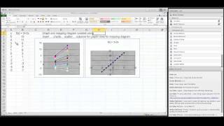
In this mini-course participants will learn how to use mapping diagrams (MD) to visualize functions for many calculus concepts. For a given function, f, a mapping diagram is basically a visualization of a function table that can be made dynamic with current technology. The MD represents  x  and f(x) from the table as points on parallel axes and arrows between the points indicate the function relation. The course will start with an overview of MD’s and then connect MD's to key calculus definitions and theory including: linearity, limits, derivatives, integrals, and series. Participants will learn how to use MD’s to visualize concepts, results and proofs not easily realized with graphs for both single and multi-variable calculus. Participants are encouraged to bring a laptop with wireless capability.


1.Mapping Diagrams. ¤


1.1 What is a mapping diagram?
Introduction and simple examples from the past: Napiers Logarithm


See: http://www.maa.org/press/periodicals/convergence/logarithms-the-early-history-of-a-familiar-function-john-napier-introduces-logarithms

Logarithms: The Early History of a Familiar Function - John Napier Introduces Logarithms  by Kathleen M. Clark (The Florida State University) and Clemency Montelle (University of Canterbury)
Figure 3. Modern version of Napier's diagram

1.2 Functions: Tables, Mapping Diagrams, and Graphs [Worksheet 1, 2 and 3.]
Understanding functions using tables. mapping diagrams, and graphs.


x f(x) = -2 x + 1)
3 -5
2.4 -3.8
1.8 -2.6
1.2 -1.4
0.6 -0.2
01
-0.62.2
-1.2 3.4
-1.8 4.6
-2.4 5.8
-3 7


2. Linear Functions. ¤
Linear functions are the key to understanding calculus.
[Worksheet 4 and 5.]
Linear functions are traditionally expressed by an equation like :
$f(x)= mx + b$.
Mapping diagrams for linear functions have one simple unifying feature- the focus point, determined by the numbers
$m$ and $b$, denoted here by $[m,b]$
.
     
Mapping Diagrams and Graphs of Linear Functions
Visualizing linear functions using mapping diagrams and graphs.
This is a Java Applet created using GeoGebra from www.geogebra.org - it looks like you don't have Java installed, please go to www.java.com
Notice how points on the graph pair with arrows and points on the mapping diagram.

3.Limits and The Derivative ¤
Mapping Diagrams Meet Limits and The Derivative
3.1 Limits with Mapping Diagrams and Graphs of Functions
[Worksheet 6 and 7.]
The traditional issue for limits (and continuity) of a function $f$ is whether
$$ \lim_{x \rightarrow a}f(x) = L \ and \  \lim_{x \rightarrow a}f(x) = f(a)$$.
The definition is visualized in the following examples.


 Is $$ \lim_{x \rightarrow a} 2x - 1 = 1.5? $$

 Is $$ \lim_{x \rightarrow a} 2x - 1 = 1 ? $$
     

Mapping diagrams and graphs visualize how the definition of a limit (and continuity) works for real functions.
This is a Java Applet created using GeoGebra from www.geogebra.org - it looks like you don't have Java installed, please go to www.java.com
Compare with current GeoGebra Version 5.0.xxx 3D

Notice how points on the graph pair with the points and arrows on the mapping diagram.

3.2 The derivative of $f$ at $a$ is a number, denoted $f'(a)$, defined as a limit of ratios ( average rates or slopes of lines). i.e.,
$$f '(a) = \lim_{x \to a} \frac{f(x)-f(a)}{x-a} \ or\ f'(x) = \lim_{\Delta x \to 0}\frac {f(x+\Delta x) - f(x)}{\Delta x}$$
Four Steps: I. Evaluate: $f(x+\Delta x)$ and $f(x)$
II. Subtract: $\Delta y =f(x+\Delta x) - f(x)$
III. Divide: $\frac {\Delta y}{\Delta x} =\frac {f(x+\Delta x) - f(x)}{\Delta x}$ and simplify if possible.
IV. THINK: As $\Delta x \to 0$, does $\frac {f(x+\Delta x) - f(x)}{\Delta x} \to L$ ? If so, then $L =f'(x)$


The derivative can be visualized using a tangent line on a graph or a focus point and derivative "vector" on a mapping diagram.


The derivative can also be understood as the magnification factor of the best approximating linear function.¤
This is a Java Applet created using GeoGebra from www.geogebra.org - it looks like you don't have Java installed, please go to www.java.com
The derivative is visualized using focus points and derivative "vectors" on a mapping diagram.


In context of Sensible Calculus Text:  SC.I.B [Motivation] Estimating Instantaneous Velocity

3.3 Mapping Diagrams for Composite (Linear) Functions ¤
This is the fundamental concept for the chain rule.


Visualizing the composition of linear functions using mapping diagrams.

Composition visualized with GeoGebra.
  This is a Java Applet created using GeoGebra from www.geogebra.org - it looks like you don't have Java installed, please go to www.java.com


 3.4. Intermediate Value theorem and Newton's Method.
¤
3.4.1. Continuity can be understood by connecting it to the Intermediate Value Theorem (IVT) and solving equations of the form $f(x) = 0$.
IVT: If $f$ is a continuous function on the interval $[a,b]$ and $f(a) \cdot f(b) \gt 0$ then there is a number $c \in (a,b)$ where $f(c) = 0$.
Mapping diagrams provide an alternative visualization for the IVT. They can also be used to visualize a proof of the result using the "bisection method."

Bisection and IVT vizualized with GEOGEBRA.
This is a Java Applet created using GeoGebra from www.geogebra.org - it looks like you don't have Java installed, please go to www.java.com

3.4.2 An early application of the first derivative, Newton's method for estimating roots of functions is visualized with mapping diagrams.
¤


The first step of Newton's method for estimating roots visualized with a mapping diagram
using the derivative focus point to find $x_1$
$x_{n+1} =x_n - f(x_n)/f'(x_n)$ $f(x)=x^2- 2$ $f'(x)=2x$
$f(x)/f'(x) =(x^2 - 2) / (2x)$
3.00000000000000 7.00000000000000 6.00000000000000 1.16666666666667
1.83333333333334 1.36111111111111 3.66666666666667 0.371212121212122
1.46212121212121 0.137798438934803 2.92424242424243 0.0471227822264093
1.41499842989480 0.00222055660475729 2.82999685978961 0.000784649847605263
1.41421378004720 6.15675383563997E-7 2.82842756009440 2.17674085859724E-7
1.41421356237311 4.75175454539568E-14 2.82842712474623 1.67999893079162E-14
1.41421356237310 -4.44089209850063E-16 2.82842712474619 -1.57009245868378E-16
1.41421356237310 4.44089209850063E-16 2.82842712474619 1.57009245868378E-16
1.41421356237310 -4.44089209850063E-16 2.82842712474619 -1.57009245868378E-16


This is a Java Applet created using GeoGebra from www.geogebra.org - it looks like you don't have Java installed, please go to www.java.com


3.5. 1st Derivative Analysis ¤
The traditional analysis of the first derivative is visualized with mapping diagrams. Extremes and critical numbers and values are connected. Time permitting- Visualize the Mean Value Theorem (MVT).

3.5.1 First Derivative Analysis. Visualizing the derivative for an interval with the "derivative vector" in a mapping diagram supports first derivative analysis for monotonic function behavior.
¤
        
Mapping Diagram Examples: $1:x^2; 2: 3x^2-2x^3 ; 3: 2x^3-3x^2; 4: \sin(\frac {\pi}2 x)$
  This is a Java Applet created using GeoGebra from www.geogebra.org - it looks like you don't have Java installed, please go to www.java.com
Graphs of functions and mapping diagrams visualize first derivative analysis.

3.5.2 Using acceleration to interpret the second derivative connects the second derivative analysis to the (rate of) change of the derivative.¤
If $f''(x) \gt 0$  for an interval then $f'(x)$ is increasing for that interval and $f(x)$ is accelerating for that interval.


This is a Java Applet created using GeoGebra from www.geogebra.org - it looks like you don't have Java installed, please go to www.java.com
Notice how the points on the graph are paired with the arrows on the mapping diagram.


3.5.3 First and Second Derivative Analysis. Visualizing the derivative for an interval with the "derivative vector" in a mapping diagram supports first derivative analysis for extremes, critical numbers and values, and the first and second derivative tests.¤
Mapping Diagram and Graphs for First and Second Derivative Analysis Examples
  This is a Java Applet created using GeoGebra from www.geogebra.org - it looks like you don't have Java installed, please go to www.java.com

4 Differentials, Differential Equations, and Euler's Method ¤
The major connection between the derivative and the differential is visualized by a mapping diagram. 

4.1.1 Mapping Diagrams for the Differential
The differential essentially uses the best linear approximation interpretation of the derivative to estimate the values of the function for small changes, $dx$, near a known value, $ x=a$ by adding $dy = f'(a) * dx$ to $f(a)$. So $$f(a+dx) \approx f(a)+dy = f(a) + f'(a)dx$$,


GeoGebra: Mapping Diagram for the Differential
Compared with The Graphical Interpretation of the Differential
GG Applet This is a Java Applet created using GeoGebra from www.geogebra.org - it looks like you don't have Java installed, please go to www.java.com

Notice how the points on the graph are paired with the points and arrows on the mapping diagram.        

4.1.2 Using acceleration connects the second derivative analysis to "concavity" and estimation concepts for the differential.


4.2 Differential Equations, Euler, Mapping Diagrams ¤
4.2.1Iterating the differential gives a numerical tool (Euler's Method) for estimating the solution to an initial value problem for a differential equation.
$P(x,y)= \frac {dy}{dx}, f(a)=c$

x f(x) f'(x) = 2x - y
df=f'(x)dx
02.-2. -0.5
0.25 1.5 -1.-0.25
0.5 1.25-0.25-0.0625
0.751.18750.31250.078125
1.1.265625

Mapping Diagram Visualizes Estimate of Solution of Initial Value Problem by Euler's Method

This is a Java Applet created using GeoGebra from www.geogebra.org - it looks like you don't have Java installed, please go to www.java.com

Estimate $f(b)$ given $y'= P(x,y)$ and $f(a)=c$ in N steps.
$ \Delta x = \frac{b-a}N;  f(b) \approx f(a) + \sum_{k=0}^{k=n-1} P(x_k,y_k)\Delta x $
In Context of Sensible Calculus Text: IV.E Euler's Method ¤