The Door Swings Both Ways:
Making Calculus Sensible with Economics
 or
Economics Sensible with Calculus.
Best viewed with Netscape 6.0 or higher.


Abstract:
General calculus textbooks often refer to economics in a limited role as an application. Professor Flashman will discuss using economics systematically in a calculus program to enhance the understanding of differential and integral calculus. He will also illustrate the distinction between arguments based on reasoning about economics and those based on mathematics.
Preface: A traditional approach to calculus uses two interpretations for most of the calculus concepts: An additional interpretation based on economics concepts provides a strong alternative that has the advantage of integrating the business/economics issues of marginal rates that are basic to most economics with the mathematical concepts of the calculus.

Though economics is presented only occasionally in calculus books in a single section or two, no current traditional calculus text has treated the economics marginal concepts as an interpretation or application that presents the calculus concepts consistently along with those of economics.

This work is connected toThe Sensible Calculus Program.

Below are several examples illustrating how economics concepts can work as interpretations compared with the more traditional interpretations.
For this presentation I will concentrate on a few of these examples:

1.
Why exp'(x) = exp(x): Using economics to understand.
2. Marginal Concepts: Understanding the analysis of critical points. The door swings both ways.
3.
The Evaluation Form of Fundamental Theorem of Calculus. Marginal concepts, the differential, and Euler's Method.
4. The Derivative Form of the Fundamental Theorem of Calculus  and Applications of the Definite Integal.


1. Using economics to understand informally why exp'(x) = exp(x). [Economics helps make math sensible.]

Recall that there is a relation between the exponential function with the base e and continuously compound interest.

This is based on the characterization  of e by the estimation with [1+1/u]u when u is a large number.

The economic context: I invest an amount (the principle, P) to be paid interest at an annual rate of r = 100r % . The interest could be
  1. paid only at the date of withdrawal (called simple interest), or 
  2. compounded n times a year, or 
  3. compounded continuously.
I would like to know in each case:
How much I will have after t years where t can be any reasonable part of a year?

 
Analysis 1:For interest paid only at the date of withdrawal. The value S of a principle P with interest paid only at the date of withdrawal t part of a year is given by
S(t)= P + Prt = P(1+rt). (1)
Notice: This is a linear function of t,  with slope or rate Pr.
Analysis 2:For interest compounded n times a year.
The value A of a principle P compounded n times annually at an annual rate of r for t = k /n parts of a year is given by
A(t)= P*(1+r/n)k. (2)
Notice: This is a discrete exponential function of k, with base b=(1+r/n).
The increment in value for the first period is precisely Pr/n.
So the rate for the first period of compounding is (Pr/n) / (1/n) =Pr.


Analysis 3:For interest compounded continuously.

We use the previous analysis to estimate. The value A of a principle P compounded n times annually at an annual rate of r for t = k /n parts of a year was given by
A(t)= P*(1+r/n)k. (2)

Letting u = n/r , we have 1/u = r/n.

Note that k = t n
  and we have
A(t)= P (1+ 1/u)urt = P*((1+ 1/u)u)rt .     (2*)

By considering compounding a large number of times per year, we estimate continuously compounding interest.

When n is large, so is u,
and we have A(t) is approximately P*
ert.  This gives the value for the limiting continously compunded value:
A(t) = P* ert .   (3)

Notice:
This is a continuous exponential function of t, with base e.
The increment in value for the first very short period of t=1/n  with n large is approximately Pr/n = Prt.
So the rate for the first period of compounding is approximately
(Pr/n) / (1/n) = Pr.  (4)
This last statement says the rate for any initial short period is approximately the same and equal to the simple (linear) interest rate of case 1!

We can now simplify this by assuming that I invested the value of 1 unit.
So in the last case at a rate of r per year compounded continously, the value at time t years is given by
A(t) = ert .

Note: When r = 1, the formula tells us that for continously compounding A is the natural exponential function, A(t) = exp(t) =
et .
Now for the calculus:

First, we notice that for any exponential function f (x) = b
t = exp(rx) =erx ,
f ' (x) = f (x)* f '(0).
This is a direct result of the fact about exponents:
[er(x+h) - erx ]/h = erx * [erh - 1]/h

and f ' (0) is the slope of the line tangent to the graph of f  at x= 0.
So to find exp'(x) we need only show that exp'(0)=1.

So we need to find the limit as h approaches 0 for
[eh - 1]/h.

Now we can turn to our economic analysis for help. We think of the context of continuously compounding with a principal of P = 1 and rate r = 1.
Thus A(t) =
et .
For a small h value we use h = 1/n where n is a large natural number. The economic estimates
for the rate of change for the first period of compounding corresponds precisely to the estimation of [eh - 1]/h.
But the economic interpretation said that for any estimation of h this rate would be the same, Pr = 1.
So  exp'(0) = 1 and exp'(x) = exp(x).

Notice that the same reasoning applied to the estimated rate in (4) can be used to show that for f (x) = exp(rt), f '(x) = r
exp(rt).

2. Marginal Concepts: Understanding the analysis of critical points.

A comparison of position vs. profit
Generic Example(s) and Precalculus concepts: Functions and Rates.
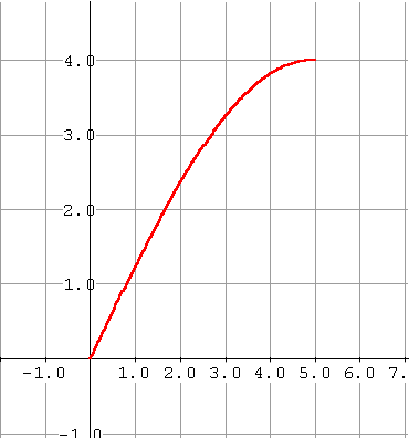
Measurement of position of an object.
Measurement of Production and Sales of Goods or Services.
Position functions. y = s(t)
(Cumulative) Profit functions.
y = P(x) = Profit [revenue or cost]for producing x units.
x measures the production or sales level.

.
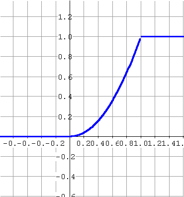
Constant velocity
∆s(t) = k t
Uniform (Constant per unit) profit functions
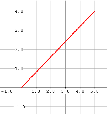
∆P(x) = k x
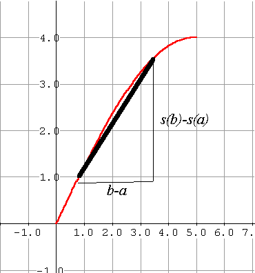
Average velocity over the interval [a,b]
v[a,b] = [s(b)-s(a)]/ [b-a]
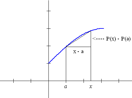
Average Marginal Profit for x for the interval [a,b
AP[a,b] = [P(b)-P(a)]/ [b-a]


 The Derivative.
Position functions determine velocity functions as limits of average velocity.
Profit functions determine marginal profit functions as limits of average marginal profit.
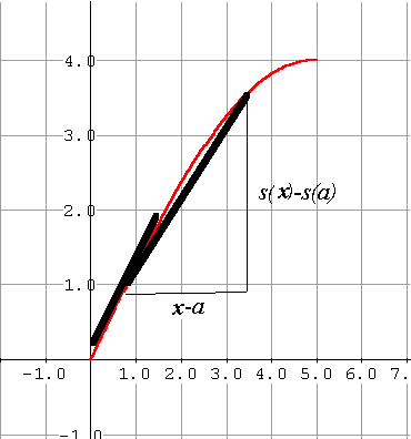
Instantaneous velocity at the point x=a
v(a) = lim [s(x)-s(a)] / [x - a]
                         xa
Marginal Profit for x at x=a
P'(a) = MP(a) = lim [P(x)-P(a)]/ [x-a]
                                     xa
 
Constant Multiple and Sum Rules:
M(a P(x)) = a MP(x)
Change in monetary scale measuring profits.

C(x) = C1(x) + C2(x), then
MC(x) = MC1(x) + MC2(x)

If cost has two components,
then the marginal cost is the sum of the marginal costs of those components.

P= R-C
MP = MR - MC.

The marginal profit is composed of the marginal revenue less the marginal cost.

Product and Quotient Rules:
R = p*x
dR/dt = x*dp/dt + p*dx/dt

The rate at which revenues change with respect to time is determined by the rate at which the price is changing and the rate at the level of sales is changing.

AvP = P/x  so  
MAvP = MP/x - P/x2 = MP/x - AvP/x =
[MP - AvP]/x
The Marginal average price is determined by the average of the marginal price less the average price.

Chain Rule:

dR/dt = dR/dx * dx/dt = MR * dx/dt

The rate of change of revenue over time is determined by the product of the marginal revenue and the rate at which the level of sales are changing.


Analysis of the first derivative
Position moving up-increasing: ds/dt >0
Position moving down- decreasing: ds/dt <0
Profit moving up-increasing: dP/dx >0
Profit moving down- decreasing: dP/dx <0
Extreme position. ds/dt = 0
Extreme profit: dP/dx = 0
Applications  
Maximaizing Profit: Since P = R- C. A necessary condition for maximal profit is that MR = MC.

Maximizing Revenues:

Suppose a relation between price (p) and sales (x) ... usually described as "the demand curve."
R = p*x
So
dR/dx = p + x * dp/dx.
So maximal revenues occur when  0 = p + x * dp/dx

or

-x/p*dp/dx = 1
or from the differential point of view  when
dx/x = -dp/p.
From an economics point of view:
-x/p*dp/dx  =  - [dp/p]/[dx/x]  is called the elasticity of demand...

indicating the relation of a percentage change in price to a percentage change in sales.

The economic statement
:  A necessary condition to achieve maximal revenues at a given price is that the elasticity of demand at that price must be 1.
The economic argument: If not so,  then one can adjust the price up or down to improve revenues since a greater or lesser price by a small percentage will give larger or smaller percentage change in sales and thus larger revenues.


The Mean Value Theorem: At some point in time the instantaneous velocity is the average velocity
.

Mean velocity :If s is continuous on [a,b] and differentiable on (a,b) then there is a time t* where v(t*)=[s(b)-s(a)]/[b-a]
Average Profit: If P is continuous on [a,b] and differentiable on (a,b) then there is a level of production x* where MP(x*)=[P(b)-P(a)]/[b-a]


3. Marginal Concepts, The Differential, Euler's Method and the Evaluation Form of Fundamental Theorem of Calculus, and Differential Equations.

Differential Equations

Initial Value Problems: Given velocity as a function of time and an initial position, find the position as a function of time.
Given  v(t)=s'(t) and s(0)=a. Find s(t).
Initial Value Problems: Given the marginal cost as a function of the level of production x and the fixed costs, find the cost as a function of the level of production.

Given f (x) = C'(x) with C(0) = C0. Find C(x).
Euler's Method interpreted as estimating the position based on the velocity function and the initial position.
Euler's Method interpreted as estimating the cost based on the marginal cost function and the fixed cost.
Use Euler to estimate the net change in position s for a time interval [a,b].  
By definition, Euler also estimates

ab  v(t) dt .
So ... = s(b) - s(a).
Use Euler to estimate the net change in costs C for a production interval [a,b].
By definition,  Euler also estimates
 
ab MC(x) dx .
So ... = C(b) - C(a).
Application- Qualitative Analysis related to a Differential Equation
The Evans Price Adjustment Model:
If the price is not at equilibrium,
then it will change over time so that its rate of change, dp/dt, is proportional to the shortfall, that is
dp/dt = k (D(p) -S(p)).


  4.The Derivative Form of the Fundamental Theorem of Calculus


The Integral: Understanding the Fundamental Theorem of Calculus
Velocity determines the net change in position functions.  
s(t) - s(a) = at  v(t) dt
If  s(x) = ax  v(t) dt  
then  s'(x) =  v(x).
Marginal Cost functions determine the net change in Cost functions.
C(b) - C(a) = abMC(x) dx .
If C(x) = ax  MC(t) dt
then  C'(x) = MC(x).
The mean value theorem for integrals.
If v is continuous on [a,b] there is some t* where
v(t*)[b-a] = [s(b)-s(a)] = ab  v(t) dt
 
The mean value theorem for integrals.
If  MC is continuous on [a,b] there is some t*
where

MC(t*)[b-a] = [C(b)-C(a)] = ab  MC(t) dt
The average value of the velocity is 
ab  v(t) dt/[b-a].
The average value of the marginal cost is 
ab  MC(x) dx/[b-a].
Integration Applications:
Consumer Savings and Producer Surplus
Future and present value.

The End

The Sensible Calculus

http://flashman.neocities.org

flashman@humboldt.edu