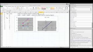
Figure 3. The relation between the two lines and the logs and sines
Linear Functions.
Understanding functions using tables. mapping diagrams and graphs.
Functions: Tables, Mapping Diagrams, and Graphs
2. Linear Functions. ¤
Linear functions are the key to understanding calculus.
Linear functions are traditionally expressed by an equation like : $f(x)= mx + b$.
Mapping diagrams for linear functions have one simple unifying feature- the focus point, determined by the numbers $m$ and $b$, denoted here by $[m,b]$.
Mapping Diagrams and Graphs of Linear Functions
Visualizing linear functions using mapping diagrams and graphs.
Notice how points on the graph pair with arrows and points on the mapping diagram.
3.Limits and The Derivative ¤ Mapping Diagrams Meet Limits and The Derivative
3.1 Limits with Mapping Diagrams and Graphs of Functions
The traditional issue for limits of a function $f$ is whether $$ \lim_{x \rightarrow a}f(x) = L$$.
The definition is visualized in the following example.
Mapping diagrams and graphs visualize how the definition of a limit works for real functions.
Notice how points on the graph pair with the points and arrows on the mapping diagram.
3.2 The derivative of $f$ at $a$ is a number, denoted $f'(a)$, defined as a limit of ratios (
average rates or slopes of lines). i.e., $$f'(a) = \lim_{x \rightarrow a} \frac {f(x)-f(a)}{x-a}.$$
The derivative can be visualized using a tangent line on a graph or a focus point and derivative "vector" on a mapping diagram.
The derivative can also be understood as the
magnification factor of the best linear approximating function.¤
The derivative can be visualized using focus points and derivative "vectors" on a mapping diagram.
3.3 Mapping Diagrams for Composite (Linear) Functions ¤
This is the fundamental concept for the chain rule.
Visualizing the composition of linear functions using mapping diagrams.
3.4. Intermediate Value theorem and Newton's method.
3.4.1. Continuity can be understood by connecting it to the Intermediate
Value Theorem (IVT) and solving equations of the form $f(x) = 0$.
IVT: If $f$ is a continuous function on the interval $[a,b]$ and $f(a)
\cdot f(b) \gt 0$ then there is a number $c \in (a,b)$ where $f(c) = 0$.
Mapping diagrams provide an alternative visualization for the IVT. They
can also be used to visualize a proof of the result using the "bisection
method."
Insert GEOGEBRA for Bisection and IVT.
3.4.2 An early application of the first derivative, Newton's method for estimating roots of functions is visualized with
mapping diagrams.
The first step of Newton's method for estimating roots visualized with a mapping diagram
using the derivative focus point to find $x_1$
The traditional analysis of the first derivative is visualized with
mapping diagrams. Extremes and critical numbers and values are connected.
Time permitting- Visualize the Mean Value Theorem (MVT).
3.5.1 First Derivative Analysis. Visualizing the derivative for an
interval with the "derivative vector" in a mapping diagram supports
first derivative analysis for monotonic function behavior.
Graphs of functions and mapping diagrams visualize first derivative analysis.
3.5.2 Using
acceleration to interpret the second derivative connects the second
derivative analysis to the (rate of) change of the
derivative.
If $f''(x) \gt 0$ for an interval then $f'(x)$ is increasing for
that interval and $f(x)$ is accelerating for that interval.
Notice how the points on the graph are paired with the arrows on the mapping diagram.
3.5.3 First and Second Derivative Analysis. Visualizing the derivative
for an interval with the "derivative vector" in a mapping diagram
supports first derivative analysis for extremes, critical numbers and values, and
the first and second derivative tests. [See previous figure.]
Mapping Diagram and Graphs for First and Second Derivative Analysis Examples
Mapping Diagram and Graph for First and Second Derivative Analysis
4Differentials, Differential Equations, and Euler's Method ¤
The major connection between the derivative and the differential is
visualized by a mapping diagram.
4.1.1 Mapping Diagrams for the Differential
Mapping Diagram for the Differential
Notice how the points on the graph are paired with the points and arrows on the mapping diagram.
4.1.2 Using acceleration connects the second derivative analysis to "concavity" and estimation concepts for the differential.
4.2 Differential Equations, Euler, Mapping Diagrams ¤ Iterating the differential gives a
numerical tool (Euler's Method) for estimating the solution to an
initial value problem for a differential equation.
$P(x,y)= \frac {dy}{dx}, f(a)=c$
Estimate $f(b)$ given $y'= P(x,y)$ and $f(a)=c$ in N steps. $ \Delta x = \frac{b-a}N; f(b) \approx f(a) + \sum_{k=0}^{k=n-1} P(x_k,y_k)\Delta x $


 AMATYC Webinar Martin Flashman - Using Mapping Diagrams to Understand Functions (YouTube)
 AMATYC Webinar M Flashman Using Mapping Diagrams to Understand Trig Functions (YouTube)
 Martin Flashman ...Solving Linear Equations Visualized with Mapping Diagrams (YouTube)
 Martin Flashman ...Partial Derivatives: An Introduction Using Mapping Diagrams (You Tube)