HSU Mathematics Department Colloquium
¤
Feb. 5, 2015 Mapping Diagrams Take on Calculus and Complex Variables
Martin Flashman
Professor of Mathematics
Humboldt State University
Link for these notes: http://flashman.neocities.org/Presentations/MD.HSU.2_5_15.html
Abstract:
Visualizing functions with mapping diagrams has been a recurrent theme and a central passion for me over many years.
In this presentation I'll demonstrate some of my more recent assaults on
the challenges of differential and integral calculus and even the study
of functions of a complex variable using mapping diagrams.
Knowledge of at least one semester of calculus will be presumed.
Background and References on Mapping Diagrams ¤
What is a mapping diagram?
Introduction and simple examples from the past: Linear Functions.
Understanding functions using tables. mapping diagrams and graphs.
Functions: Tables, Mapping Diagrams, and Graphs
1.2. Linear Functions. ¤
Linear functions are the key to understanding calculus.
Linear functions are traditionally expressed by an equation like : $f(x)= mx + b$.
Mapping diagrams for linear functions have one simple unifying feature- the focus point, determined by the numbers $m$ and $b$, denoted here by $[m,b]$.
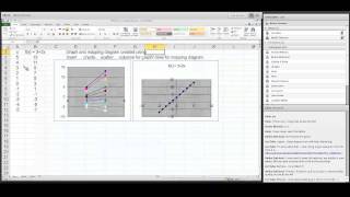
Mapping Diagrams and Graphs of Linear Functions
Visualizing linear functions using mapping diagrams and graphs.
Notice how points on the graph pair with arrows and points on the mapping diagram.
1.3.Limits and The Derivative ¤ Mapping Diagrams Meet Limits and The Derivative
1.3.1 Limits with Mapping Diagrams and Graphs of Functions
The traditional issue for limits of a function $f$ is whether $ \lim_{x \rightarrow a}f(x) = L$.
The definition is visualized in the following example.
Mapping diagrams and graphs visualize how the definition of a limit works for real functions.
Notice how points on the graph pair with the points and arrows on the mapping diagram.
1.3.2 The derivative of $f$ at $a$ is a number, denoted $f'(a)$, defined as a limit of ratios (
average rates or slopes of lines). i.e., $$f'(a) = \lim_{x \rightarrow a} \frac {f(x)-f(a)}{x-a}.$$
The derivative can also be understood as the
magnification factor of the best linear approximating function.¤
The derivative can be visualized using focus points and derivative "vectors" on a mapping diagram.
1.3.3 Mapping Diagrams for Composite (Linear) Functions ¤
This is the fundamental concept for the chain rule.
Visualizing the composition of linear functions using mapping diagrams and graphs.
Notice how points on the graph are paired with the points and arrows on the mapping diagram.
1.4.1st Derivative Analysis ¤
The traditional analysis of the first derivative is visualized with
mapping diagrams. Extremes and critical numbers and values connected.
Time permitting- the Intermediate and Mean Value Theorems are
visualized- along with Newton's Method for estimating roots to an
equation.
1.4.1 First [and Second] Derivative Analysis.
Graphs of functions and mapping diagrams visualize first and second derivative analysis.
Notice how the points on the graph is paired with the points on the mapping diagram.
1.5.Differentials, Differential Equations, and Euler's Method ¤
The major connection between the derivative and the differential is
visualized by a mapping diagram.
1.5.1 Mapping Diagrams for the Differential
Mapping Diagram for the Differential
Notice how the points on the graph are paired with the points and arrows on the mapping diagram.
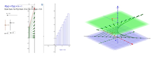
1.5.2 Differential Equations, Euler, Mapping Diagrams ¤ Iterating the differential gives a
numerical tool (Euler's Method) for estimating the solution to an
initial value problem for a differential equation.
$P(x,y)= \frac {dy}{dx}, f(a)=c$
Estimate $f(b)$ given $y'= P(x,y)$ and $f(a)=c$ in N steps. $ \Delta x = \frac{b-a}N; f(b) \approx f(a) + \sum_{k=0}^{k=n-1} P(x_k,y_k)\Delta x $
1.6.Integration and the Fundamental Theorem ¤
Connecting Euler's method to sums leads to a visualization of the
definite integral as measuring a net change in position in a mapping
diagram and an area of the graph of the velocity. Definition: As $N \rightarrow \infty$ $\sum_{k=0}^{k=n-1} P(x_k)\Delta x \rightarrow \int_a^b P(x)dx$ The Fundamental
Theorem of Calculus.Suppose $y = P(x) = f'(x)$ is a continuous function, then
$\int_a^b P(x)dx + f(a) = f(b)$
or
$\int_a^b P(x)dx = f(b) - f(a)$
where $f'(x) = P(x)$.
1.6.1 Euler's Method visualized with mapping diagram and graph, showing
the connection between the mapping diagram and the area of a region in
the plane bounded by the graph of
$y = P(x) = f'(x)$, the X axis, X=a and X
= b.
Move the sliders to change a,b, and N. You can also change the function P(x) = f'(x) by entering a new function in the box.
Mapping diagrams visualize functions of complex variables in new ways
that illustrate some important functions.
Examples using linear functions, linear fractional (Moebius), and power functions. 2.1.1 A complex linear function can be visualized as a mapping from C to C. Mapping Diagram for Complex Linear Function (Circles) This example shows a linear function on a single complex number and points on a circle in the complex plane.
Use the slider to change the radius of the circle, r, in the domain for the mapping diagram. 2.1.2 Complex Mapping Diagram of Linear Function (lines) ¤
A complex linear function can be visualized as a mapping from C to C.
This example shows a linear function on a single complex number and points on a line in the complex plane.
You can move the point z#, change the slider to move the line, and enter new function. 2.1.3 Visualizing Complex Moebius Functions with Mapping Diagrams ¤
You can move a,b,and c in the Graphics window to change the complex parameters for the Moebius function.
The sliders adjust the height of the second complex plane and the radius of the circle for the mapping diagram arrow source.
2.1.4 Visualizing Complex Power Functions with Mapping Diagrams ¤
The
sliders adjust the height of the second complex plane, the power, n,
and the radius of the circle for the mapping diagram arrow source.