Home
Center for Recruitment and Retention of Mathematics Teachers
University of Arizona
  ¤
November 8, 2017

Using Mapping Diagrams to Make Sense of Functions and Calculus
Part II
Linearity, Limits, Derivatives,Differential Equations, and Integration
  
Martin Flashman
Professor of Mathematics
Humboldt State University


http://flashman.neocities.org/Presentations/CRR2017/MD.LINKS.II.html


Abstract:
Participants will learn how to use mapping diagrams (MD) to make sense of functions and relate these to materials taught in calculus and in preparing for calculus.
A mapping diagram is an alternative to a Cartesian graph that visualizes a function using parallel axes. Like a table, it can present finite date, but also can be used dynamically with technology.
An overview of basic function concepts with MD’s will begin the session using worksheets and GeoGebra.
Connections of MD's to key concepts in studying calculus and preparing to study calculus will follow showing the power of MD’s to make sense of function concepts of measurement, rate, composition, and approximation related to calculus.

Background and examples will be available at Mapping Diagrams from A(lgebra) B(asics) to C(alculus) and D(ifferential) E(quation)s. A Reference and Resource for Function Visualizations Using Mapping Diagrams. http://flashman.neocities.org/MD/section-1.1VF.html


Outline for Workshop II  ¤
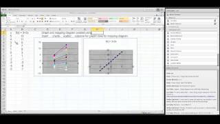
  • Mapping Diagrams
    • What is a Mapping Diagram? Review
    • Brief reports on use Workshop I
  • Linear Functions
    • Linear functions are the key to understanding calculus.
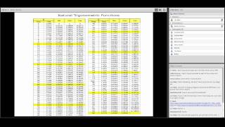
    • Nonlinear ( 1/x, trig, exp/ln) Connect to Resource
  • Limits and The Derivative (visualize rate/ratio)
    • An On-line Lesson on the Derivative
    • Limits with Mapping Diagrams
    • The Derivative As A
      • Number,
      • Magnification
      • Rate
      • Vector
    • The Chain Rule: Mapping Diagrams for Composite (Linear) Functions
      • An On-line Lesson on the Chain Rule
    • Continuity and Solving Equations
      • The Intermediate Value Theorem
      • Newton's Method.
    • 1st and 2nd Derivative Analysis [Time permitting]
  • Differentials, Differential Equations, and Euler's Method
    • Mapping Diagrams for the Differential
    • Differential Equations, Euler, Mapping Diagrams
  • Integration, the Fundamental Theorem(s) of Calculus, and Applications to Area.


1.Mapping Diagrams. ¤

1.2 Functions: Tables, Mapping Diagrams, and Graphs [Worksheet 1a and b, 2a and b, and 3a, b, and c.] ¤


1.3 Technology Examples  ¤


2. Linear (and Quadratic) Functions. ¤

2.3 Linear functions are the key to understanding calculus.[Worksheet II 1 and 2]
¤
Linear functions are traditionally expressed by an equation like :
$f(x)= mx + b$.
Mapping diagrams for linear functions have one simple unifying feature- the focus point, determined by the numbers
$m$ and $b$, denoted here by $[m,b]$
.
     
Mapping Diagrams and Graphs of Linear Functions
Visualizing linear functions using mapping diagrams and graphs.
This is a Java Applet created using GeoGebra from www.geogebra.org - it looks like you don't have Java installed, please go to www.java.com
Notice how points on the graph pair with arrows and points on the mapping diagram.


2.4 Nonlinear ( 1/x, trig, exp/ln) ¤  
For examples: Change functions in previous examples or connect to
Mapping Diagrams from A(lgebra) B(asics) to C(alculus) and D(ifferential) E(quation)s.


3.Limits and The Derivative ¤
Mapping Diagrams Meet Limits and The Derivative

3.0 An On-line Lesson on the Derivative
Go to Underground Mathematics (University of Cambridge):

mapping-a-derivative
With a partner start work on the Problem:
[You can use the GeoGebra applet on the linked web page.]


3.1 Limits with Mapping Diagrams
[Worksheet II 3a and b.]  ¤
The traditional issue for limits (and continuity) of a function $f$ is whether
$$ \lim_{x \rightarrow a}f(x) = L \ and \  \lim_{x \rightarrow a}f(x) = f(a)$$.
The definition is visualized in the following examples.
What is important even without the limit concept is the visualization of related inequalities:
Find $\delta$ so that if $a-\delta < x < a+ \delta$, then $L - \epsilon < f(x) < L+\epsilon$.
More specifically- in a linear example:  Find $\delta$ so that if $1-\delta < x < 1+ \delta$, then $1 - 0.5 < 2x-1 < 1+ 0.5$.


 Is $$ \lim_{x \rightarrow a} 2x - 1 = 1.5? $$

 Is $$ \lim_{x \rightarrow a} 2x - 1 = 1 ? $$
     

Mapping diagrams and graphs visualize how the definition of a limit (and continuity) works for real functions.

Notice how points on the graph pair with the points and arrows on the mapping diagram.

3.2 The Derivative As A Number, Magnification, Rate Or Vector: [Worksheet II 4.]  ¤
The derivative of $f$ at $a$ is a number
, denoted $f'(a)$, defined as a limit of ratios ( average rates or slopes of lines). i.e.,
$$f '(a) = \lim_{x \to a} \frac{f(x)-f(a)}{x-a} \ or\ f'(x) = \lim_{\Delta x \to 0}\frac {f(x+\Delta x) - f(x)}{\Delta x}$$
Four Steps: I. Evaluate: $f(x+\Delta x)$ and $f(x)$
II. Subtract: $\Delta y =f(x+\Delta x) - f(x)$
III. Divide: $\frac {\Delta y}{\Delta x} =\frac {f(x+\Delta x) - f(x)}{\Delta x}$ and simplify if possible.
IV. THINK: As $\Delta x \to 0$, does $\frac {f(x+\Delta x) - f(x)}{\Delta x} \to L$ ? If so, then $L =f'(x)$


The derivative can be visualized using a tangent line on a graph or a focus point and derivative "vector" on a mapping diagram.


The derivative can also be understood as the magnification factor of the best approximating linear function.¤
This is a Java Applet created using GeoGebra from www.geogebra.org - it looks like you don't have Java installed, please go to www.java.com
The derivative is visualized using focus points and derivative "vectors" on a mapping diagram.


In context of Sensible Calculus Text:  SC.I.B [Motivation] Estimating Instantaneous Velocity

3.3 The Chain Rule: Mapping Diagrams for Composite (Linear) Functions
[Worksheet II 5.] ¤
This is the fundamental concept for the chain rule.
Visualizing composite functions is a major advantage of mapping diagrams in many courses in preparation for calculus.

An On-line Lesson on the Chain Rule
Go to Underground Mathematics (University of Cambridge):
chain-mapping
With a partner start work on the Warm-Up ideas  and Problem:
[You can use the GeoGebra applet in the Interactivity tab.]


Visualizing the composition of linear functions using mapping diagrams.

Composition visualized with GeoGebra.
  This is a Java Applet created using GeoGebra from www.geogebra.org - it looks like you don't have Java installed, please go to www.java.com


 3.4. Continuity and Solving Equations.
The Intermediate Value Theorem and Newton's Method.
¤
3.4.1. Continuity can be understood by connecting it to the Intermediate Value Theorem (IVT) and solving equations of the form $f(x) = 0$.
IVT: If $f$ is a continuous function on the interval $[a,b]$ and $f(a) \cdot f(b) \gt 0$ then there is a number $c \in (a,b)$ where $f(c) = 0$.
Mapping diagrams provide an alternative visualization for the IVT. They can also be used to visualize a proof of the result using the "bisection method."
[Worksheet II 6.]
The bisection method for solving equations is a technique that can be introduced in courses preparing for calculus- as soon as square roots are encountered.

Bisection and IVT vizualized with GEOGEBRA.
This is a Java Applet created using GeoGebra from www.geogebra.org - it looks like you don't have Java installed, please go to www.java.com


3.4.2 An early application of the first derivative, Newton's method for estimating roots of functions is visualized with mapping diagrams.
¤
Note: A variant of this method that uses linear interpolation can be introduced in preparation for calculus.


The first step of Newton's method for estimating roots visualized with a mapping diagram
using the derivative focus point to find $x_1$
$x_{n+1} =x_n - f(x_n)/f'(x_n)$ $f(x)=x^2- 2$ $f'(x)=2x$
$f(x)/f'(x) =(x^2 - 2) / (2x)$
3.00000000000000 7.00000000000000 6.00000000000000 1.16666666666667
1.83333333333334 1.36111111111111 3.66666666666667 0.371212121212122
1.46212121212121 0.137798438934803 2.92424242424243 0.0471227822264093
1.41499842989480 0.00222055660475729 2.82999685978961 0.000784649847605263
1.41421378004720 6.15675383563997E-7 2.82842756009440 2.17674085859724E-7
1.41421356237311 4.75175454539568E-14 2.82842712474623 1.67999893079162E-14
1.41421356237310 -4.44089209850063E-16 2.82842712474619 -1.57009245868378E-16
1.41421356237310 4.44089209850063E-16 2.82842712474619 1.57009245868378E-16
1.41421356237310 -4.44089209850063E-16 2.82842712474619 -1.57009245868378E-16


This is a Java Applet created using GeoGebra from www.geogebra.org - it looks like you don't have Java installed, please go to www.java.com


3.5. 1st Derivative Analysis: The traditional analysis of the first derivative is visualized with mapping diagrams. Extremes and critical numbers and values are connected. Time permitting- Visualize the Mean Value Theorem (MVT). ¤
3.5.1 First Derivative Analysis. Visualizing the derivative for an interval with the "derivative vector" in a mapping diagram supports first derivative analysis for monotonic function behavior.
¤
        
Mapping Diagram Examples: $1:x^2; 2: 3x^2-2x^3 ; 3: 2x^3-3x^2; 4: \sin(\frac {\pi}2 x)$
  This is a Java Applet created using GeoGebra from www.geogebra.org - it looks like you don't have Java installed, please go to www.java.com
Graphs of functions and mapping diagrams visualize first derivative analysis.


3.5.2 Using acceleration to interpret the second derivative connects the second derivative analysis to the (rate of) change of the derivative.¤
If $f''(x) \gt 0$  for an interval then $f'(x)$ is increasing for that interval and $f(x)$ is accelerating for that interval.


This is a Java Applet created using GeoGebra from www.geogebra.org - it looks like you don't have Java installed, please go to www.java.com
Notice how the points on the graph are paired with the arrows on the mapping diagram.


3.5.3 First and Second Derivative Analysis. Visualizing the derivative for an interval with the "derivative vector" in a mapping diagram supports first derivative analysis for extremes, critical numbers and values, and the first and second derivative tests.¤
Mapping Diagram and Graphs for First and Second Derivative Analysis Examples
  This is a Java Applet created using GeoGebra from www.geogebra.org - it looks like you don't have Java installed, please go to www.java.com


4 Differentials, Differential Equations, and Euler's Method ¤
The major connection between the derivative and the differential is visualized by a mapping diagram. 

4.1.1 Mapping Diagrams for the Differential [Worksheet II 7.]
The differential essentially uses the best linear approximation interpretation of the derivative to estimate the values of the function for small changes, $dx$, near a known value, $ x=a$ by adding $dy = f'(a) * dx$ to $f(a)$. So $$f(a+dx) \approx f(a)+dy = f(a) + f'(a)dx$$,
Preparation for the use of the differential concept can be introduced as soon as rates and estimations are encountered.


GeoGebra: Mapping Diagram for the Differential
Compared with The Graphical Interpretation of the Differential
GG Applet This is a Java Applet created using GeoGebra from www.geogebra.org - it looks like you don't have Java installed, please go to www.java.com

Notice how the points on the graph are paired with the points and arrows on the mapping diagram.        

4.1.2 Using acceleration connects the second derivative analysis to "concavity" and estimation concepts for the differential.


4.2 Differential Equations, Euler, Mapping Diagrams [Worksheet II 8] ¤
4.2.1Iterating the differential gives a numerical tool (Euler's Method) for estimating the solution to an initial value problem for a differential equation.
The estimations done with Euler's method can be introduced without specific use of calculus language by referring to these equations as "rate equations."
$P(x,y)= \frac {dy}{dx}, f(a)=c$

x f(x) f'(x) = 2x - y
df=f'(x)dx
02.-2. -0.5
0.25 1.5 -1.-0.25
0.5 1.25-0.25-0.0625
0.751.18750.31250.078125
1.1.265625

Mapping Diagram Visualizes Estimate of Solution of Initial Value Problem by Euler's Method

This is a Java Applet created using GeoGebra from www.geogebra.org - it looks like you don't have Java installed, please go to www.java.com

Estimate $f(b)$ given $y'= P(x,y)$ and $f(a)=c$ in N steps.
$ \Delta x = \frac{b-a}N;  f(b) \approx f(a) + \sum_{k=0}^{k=n-1} P(x_k,y_k)\Delta x $
In Context of Sensible Calculus Text: IV.E Euler's Method ¤


5.Integration and the Fundamental Theorem
Connecting Euler's method to sums leads to a visualization of the definite integral as measuring a net change in position in a mapping diagram and an area of the graph of the velocity function.
Definition: As $N \rightarrow \infty$   $\sum_{k=0}^{k=n-1} P(x_k)\Delta x \rightarrow \int_a^b P(x)dx$

The Fundamental Theorem of Calculus.   Suppose $y = P(x) = f'(x)$ is a continuous function, then
$\int_a^b P(x)dx + f(a) = f(b)$
or
$\int_a^b P(x)dx = f(b) - f(a)$
where $f'(x) = P(x)$.


5.1 [Worksheet II 9.]
Euler's Method visualized with mapping diagram and graph, showing the connection between the mapping diagram and the area of a region in the plane bounded by the graph of

$y = P(x) = f'(x)$, the X axis, X=a and X = b.

Move the sliders to change $a,b$, and $N$. You can also change the function $P(x) = f'(x)$ by entering a new function in the box. ¤


5.2 Properties of The Definite Integrals [If time permits.] [Worksheet II 10, 11, and 12.]

Additivity: $\int_a^c \ P(x ) \ dx+ \int _c^b \ P(x)\ dx\ =\ \int_a^c \ P(x)\ dx$
Scalar Multiplication: $\int_a^b  \alpha \ P(x ) \ dx =\  \alpha \int_a^b \ P(x)\ dx$
The Mean Value Property for Integrals: \int_a^b \ P(x ) \ dx =\  P(c) cdot (b-a)$


Thanks for participating
¤.