Center for Recruitment and Retention of Mathematics Teachers
University of Arizona ¤
October 18, 2017
Using Mapping Diagrams to Make Sense of Functions and Calculus
Part I
Functions, Equations, Linearity
What was covered and the edge of Part II.
Abstract:
Participants
will learn how to use mapping diagrams (MD) to make sense of functions
and relate these to materials taught in calculus and in preparing for
calculus.
A mapping diagram is an alternative to a Cartesian graph that visualizes
a function using parallel axes. Like a table, it can present finite
date, but also can be used dynamically with technology.
An overview of basic function concepts with MD’s will begin the session using worksheets and GeoGebra.
Connections of MD's to key concepts in studying calculus and preparing
to study calculus will follow showing the power of MD’s to make sense of
function concepts of measurement, rate, composition, and approximation
related to calculus.
Background and examples will be available at Mapping Diagrams from
A(lgebra) B(asics) to C(alculus) and D(ifferential) E(quation)s. A
Reference and Resource for Function Visualizations Using Mapping
Diagrams. http://flashman.neocities.org/MD/section-1.1VF.html
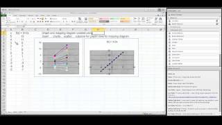
Figure 3. The relation between the two lines and the logs and sines
Written by Howard Swann and John Johnson
An early source for visualizing functions at an elementary level before calculus.
This is copyrighted material!
1.2 Functions: Tables, Mapping Diagrams, and Graphs [Worksheet 1a and b, 2a and b, and 3a, b, and c.] ¤
Understanding functions using tables. mapping diagrams, and graphs.
2. Linear (and Quadratic) Functions. ¤
2.0 An On-line Lesson on Linear Functions
Go to Underground Mathematics (University of Cambridge): mapping-a-function
Read Warm-up ONLY!
Discuss response to the two questions with partner(s).
2.1 Visualizing Linear (and Quadratic) Functions and Equations.
Solving an equation $f(x) = 0$ visualized with table and graph. [Look for graph of $f$ to cross X-axis.]
Solving an equation $f(x) = 0$ visualized with table and mapping diagram. [Look for arrow on diagram to hit $0$ on target axis.]
Main issue:
How do these visualizations connect to the algebra for solving an equation? ¤
2.2 Solving equations visualized with mapping diagrams [Worksheet 4 and 5.] *
Problems (if time permits): Use mapping diagrams to visualize the solution to the following:
A. I invested 1000 dollars in a savings account paying interest at 2%
per annum compounded continuously.In approximately how many years will
my investment grow to a value of 1500 dollars?
B. Find all angles $t$ in radians where $8\sin(2t + \pi/2)=4$.
The start of Part II
2.3 Linear functions are the key to understanding calculus.[Worksheet 6 and 7] ¤
Linear functions are traditionally expressed by an equation like :$f(x)= mx + b$.
Mapping diagrams for linear functions have one simple unifying feature- the focus point, determined by the numbers $m$ and $b$, denoted here by $[m,b]$.
Mapping Diagrams and Graphs of Linear Functions
Visualizing linear functions using mapping diagrams and graphs.
Notice how points on the graph pair with arrows and points on the mapping diagram.
3.Limits and The Derivative ¤ Mapping Diagrams Meet Limits and The Derivative
3.0 An On-line Lesson on the Derivative
Go to Underground Mathematics (University of Cambridge): mapping-a-derivative
With a partner start work on the Problem:
[You can use the GeoGebra applet on the linked web page.]
What does the mapping diagram of the function $f(x)=x^2$ look like?
What does the mapping diagram look like if it is centred on the arrow from 0
to f(0), at a scale of 1 unit per tick-mark?
What if it is centred at some other arrow, say from 1 to f(1) or −1 to f(−1) or 32 to f(32) ?
What does the mapping diagram look like if it is centred on the arrow from 1
to f(1), but this time zoomed in to 0.1 or 0.01 units per tick-mark?
What if it is instead centred on some other arrow and then zoomed in?
Can you describe what you observe?
In what ways are the mapping diagrams of the function $f(x)=x^2$
similar to those of a linear function, and in what ways are they different?
3.1 Limits with Mapping Diagrams [Worksheet 8a and b.] ¤
The traditional issue for limits (and continuity) of a function $f$ is whether $$ \lim_{x \rightarrow a}f(x) = L \ and \ \lim_{x \rightarrow a}f(x) = f(a)$$.
The definition is visualized in the following examples.
Is $$ \lim_{x \rightarrow a} 2x - 1 = 1.5? $$
Is $$ \lim_{x \rightarrow a} 2x - 1 = 1 ? $$
Mapping diagrams and graphs visualize how the definition of a limit (and continuity) works for real functions.
Notice how points on the graph pair with the points and arrows on the mapping diagram.
3.2 The Derivative As A Number, Magnification, Rate Or Vector: [Worksheet 9.] ¤
The derivative of $f$ at $a$ is a number, denoted $f'(a)$, defined as a limit of ratios (
average rates or slopes of lines). i.e.,
$$f '(a) = \lim_{x \to a} \frac{f(x)-f(a)}{x-a} \ or\ f'(x) = \lim_{\Delta x \to 0}\frac {f(x+\Delta x) - f(x)}{\Delta x}$$
Four Steps:
I. Evaluate: $f(x+\Delta x)$ and $f(x)$
II. Subtract: $\Delta y =f(x+\Delta x) - f(x)$
III. Divide: $\frac {\Delta y}{\Delta x} =\frac {f(x+\Delta x) - f(x)}{\Delta x}$ and simplify if possible.
IV. THINK: As $\Delta x \to 0$, does $\frac {f(x+\Delta x) - f(x)}{\Delta x} \to L$ ? If so, then $L =f'(x)$
The derivative can be visualized using a tangent line on a graph or a focus point and derivative "vector" on a mapping diagram.
The derivative can also be understood as the
magnification factor of the best approximating linear function.¤
The derivative is visualized using focus points and derivative "vectors" on a mapping diagram.
In context of Sensible Calculus Text:SC.I.B
[Motivation] Estimating Instantaneous
Velocity 3.3 The Chain Rule: Mapping Diagrams for Composite (Linear) Functions [Worksheet 10.] ¤
This is the fundamental concept for the chain rule.
An On-line Lesson on the Chain Rule
Go to Underground Mathematics (University of Cambridge):chain-mapping With a partner start work on the Warm-Up ideas and Problem:
[You can use the GeoGebra applet in the Interactivity tab.]
Visualizing the composition of linear functions using mapping diagrams.
Composition visualized with GeoGebra.
3.4. Continuity and Solving Equations.
The Intermediate Value Theorem and Newton's Method. ¤
3.4.1. Continuity can be understood by connecting it to the Intermediate
Value Theorem (IVT) and solving equations of the form $f(x) = 0$.
IVT: If $f$ is a continuous function on the interval $[a,b]$ and $f(a)
\cdot f(b) \gt 0$ then there is a number $c \in (a,b)$ where $f(c) = 0$.
Mapping diagrams provide an alternative visualization for the IVT. They
can also be used to visualize a proof of the result using the "bisection
method."
Bisection and IVT vizualized with GEOGEBRA.
3.4.2 An early application of the first derivative, Newton's method for estimating roots of functions is visualized with
mapping diagrams.¤
The first step of Newton's method for estimating roots visualized with a mapping diagram
using the derivative focus point to find $x_1$
$x_{n+1} =x_n - f(x_n)/f'(x_n)$
$f(x)=x^2- 2$
$f'(x)=2x$
$f(x)/f'(x) =(x^2 - 2) / (2x)$
3.00000000000000
7.00000000000000
6.00000000000000
1.16666666666667
1.83333333333334
1.36111111111111
3.66666666666667
0.371212121212122
1.46212121212121
0.137798438934803
2.92424242424243
0.0471227822264093
1.41499842989480
0.00222055660475729
2.82999685978961
0.000784649847605263
1.41421378004720
6.15675383563997E-7
2.82842756009440
2.17674085859724E-7
1.41421356237311
4.75175454539568E-14
2.82842712474623
1.67999893079162E-14
1.41421356237310
-4.44089209850063E-16
2.82842712474619
-1.57009245868378E-16
1.41421356237310
4.44089209850063E-16
2.82842712474619
1.57009245868378E-16
1.41421356237310
-4.44089209850063E-16
2.82842712474619
-1.57009245868378E-16
3.5. 1st Derivative Analysis: The traditional analysis of the first derivative is visualized with
mapping diagrams. Extremes and critical numbers and values are connected.
Time permitting- Visualize the Mean Value Theorem (MVT). ¤
3.5.1 First Derivative Analysis. Visualizing the derivative for an
interval with the "derivative vector" in a mapping diagram supports
first derivative analysis for monotonic function behavior.¤
Graphs of functions and mapping diagrams visualize first derivative analysis.
3.5.2 Using
acceleration to interpret the second derivative connects the second
derivative analysis to the (rate of) change of the
derivative.¤
If $f''(x) \gt 0$ for an interval then $f'(x)$ is increasing for
that interval and $f(x)$ is accelerating for that interval.
Notice how the points on the graph are paired with the arrows on the mapping diagram.
3.5.3 First and Second Derivative Analysis. Visualizing the derivative
for an interval with the "derivative vector" in a mapping diagram
supports first derivative analysis for extremes, critical numbers and values, and
the first and second derivative tests.¤
Mapping Diagram and Graphs for First and Second Derivative Analysis Examples
4Differentials, Differential Equations, and Euler's Method ¤
The major connection between the derivative and the differential is
visualized by a mapping diagram.
4.1.1 Mapping Diagrams for the Differential [Worksheet 11]
The differential essentially uses the best linear approximation
interpretation of the derivative to estimate the values of the function
for small changes, $dx$, near a known value, $ x=a$ by adding $dy = f'(a) * dx$ to $f(a)$. So $$f(a+dx) \approx f(a)+dy = f(a) + f'(a)dx$$,
GeoGebra: Mapping Diagram for the Differential
Compared with The Graphical Interpretation of the Differential
GG Applet
Notice how the points on the graph are paired with the points and arrows on the mapping diagram.
4.1.2 Using acceleration connects the second derivative analysis to "concavity" and estimation concepts for the differential.
4.2.1Iterating the differential gives a
numerical tool (Euler's Method) for estimating the solution to an
initial value problem for a differential equation.
$P(x,y)= \frac {dy}{dx}, f(a)=c$
x
f(x)
f'(x) = 2x - y
df=f'(x)dx
0
2.
-2.
-0.5
0.25
1.5
-1.
-0.25
0.5
1.25
-0.25
-0.0625
0.75
1.1875
0.3125
0.078125
1.
1.265625
Mapping Diagram Visualizes Estimate of Solution of Initial Value Problem by Euler's Method
Estimate $f(b)$ given $y'= P(x,y)$ and $f(a)=c$ in N steps. $ \Delta x = \frac{b-a}N; f(b) \approx f(a) + \sum_{k=0}^{k=n-1} P(x_k,y_k)\Delta x $
In Context of Sensible Calculus Text: IV.E
Euler's Method ¤